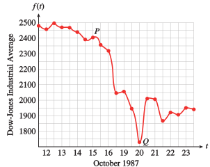
The Dow-Jones Industrial Average (DJIA) gives the average of the stock prices of 30 major companies. The graph below shows the DJIA as a function of time during the stock market correction of October 1987. The DJIA is thus \(f(t)\text{,}\) recorded at noon on day \(t\) of October.
The values of the input variable, time, are displayed on the horizontal axis, and the values of the output variable, DJIA, are displayed on the vertical axis. There is no formula that gives the DJIA for a particular day; but it is still a function, defined by its graph. The value of \(f(t)\) is specified by the vertical coordinate of the point with the given \(t\)-coordinate.
We can say that \(f(20) = 1726\text{,}\) so the point \((20, 1726)\) lies on the graph of \(f\text{.}\) This point is labeled \(Q\) in the figure above.
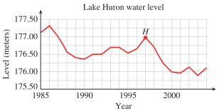
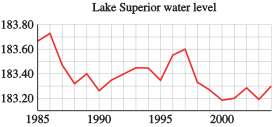
The water level in Lake Huron alters unpredictably over time. The graph below gives the average water level, \(L(t)\text{,}\) in meters in the year \(t\) over a 20-year period. (Source: The Canadian Hydrographic Service)
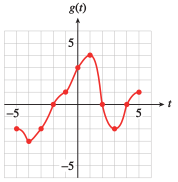
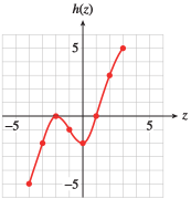
To find \(g(-2)\text{,}\) we look for the point with \(t\)-coordinate \(-2\text{.}\) The point \((-2, 0)\) lies on the graph of \(g\text{,}\) so \(g(-2) = 0\text{.}\) Similarly, the point \((5, 1)\) lies on the graph, so \(g(5) = 1\text{.}\)
We look for points on the graph with \(y\)-coordinate \(-2\text{.}\) Because the points \((-5, -2)\text{,}\)\((-3, -2)\text{,}\) and \((3, -2)\) lie on the graph, we know that \(g(-5) = -2\text{,}\)\(g(-3) = -2\text{,}\) and \(g(3) = -2\text{.}\) Thus, the \(t\)-values we want are \(-5\text{,}\)\(-3\text{,}\) and \(3\text{.}\)
The highest point on the graph is \((1, 4)\text{,}\) so the largest \(y\)-value is \(4\text{.}\) Thus, the maximum value of \(g(t)\) is \(4\text{,}\) and it occurs when \(t = 1\text{.}\)
A graph is increasing if the \(y\)-values get larger as we read from left to right. The graph of \(g\) is increasing for \(t\)-values between \(-4\) and \(1\text{,}\) and between \(3\) and \(5\text{.}\) Thus, \(g\) is increasing on the intervals \((-4, 1)\) and \((3, 5)\text{.}\)
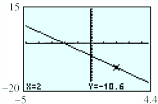
Press TRACE, and a “bug” begins flashing on the display. The coordinates of the bug appear at the bottom of the display, as shown in the figure. Use the left and right arrows to move the bug along the graph. You can check that the coordinates of the point \((2, -10.6)\) do satisfy the equation \(y = -2.6x - 5.4\text{.}\)
The points identified by the Trace bug depend on the window settings. If we want to find the \(y\)-coordinate for a particular \(x\)-value, we enter the \(x\)-coordinate of the desired point and press ENTER.
Although some functions are defined by their graphs, we can also construct graphs for functions described by tables or equations. We make these graphs the same way we graph equations in two variables: by plotting points whose coordinates satisfy the equation.
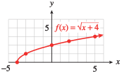
We choose several convenient values for \(x\) and evaluate the function to find the corresponding \(f(x)\)-values. For this function we cannot choose \(x\)-values less than \(-4\text{,}\) because the square root of a negative number is not a real number.
Points on the graph have coordinates \((x, f(x))\text{,}\) so the vertical coordinate of each point is given by the value of \(f(x)\text{.}\) We plot the points and connect them with a smooth curve, as shown in the figure. Notice that no points on the graph have \(x\)-coordinates less than \(-4\text{.}\)
Technology1.80Using Technology to Graph a Function.
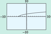
We can also use a graphing utility to obtain a table and graph for the function in Example 1.78. We graph a function just as we graphed an equation. For this function, we enter \(Y_1 = \sqrt{\,}(X+4)\) and press ZOOM\(6\) for the standard window. The graph is shown below.
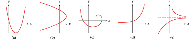
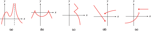
In a function, two different outputs cannot be related to the same input. This restriction means that two different ordered pairs cannot have the same first coordinate. What does it mean for the graph of the function?
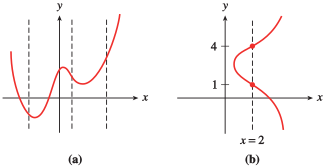
Consider the graph shown in figure (a) below. Every vertical line intersects the graph in at most one point, so there is only one point on the graph for each \(x\)-value. This graph represents a function.
In figure (b), however, the line \(x = 2\) intersects the graph at two points, \((2, 1)\) and \((2, 4)\text{.}\) Two different \(y\)-values, \(1\) and \(4\text{,}\) are related to the same \(x\)-value, \(2\text{.}\) This graph cannot be the graph of a function.
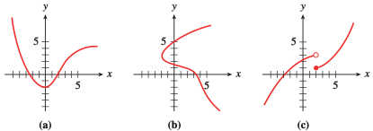
For graph (c), notice the break in the curve at \(x = 2\text{:}\) The solid dot at \((2, 1)\) is the only point on the graph with \(x = 2\text{;}\) the open circle at \((2, 3)\) indicates that \((2, 3)\) is not a point on the graph. Thus, graph (c) is a function, with \(f(2) = 1\text{.}\)
SubsectionGraphical Solution of Equations and Inequalities
The graph of an equation in two variables is just a picture of its solutions. When we read the coordinates of a point on the graph, we are reading a pair of \(x\)- and \(y\)-values that make the equation true.
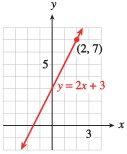
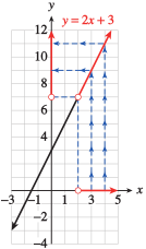
For example, the point \((2, 7)\) lies on the graph of \(~y = 2x + 3~\) shown at right, so we know that the ordered pair \((2, 7)\) is a solution of the equation \(y = 2x + 3\text{.}\) You can verify algebraically that \(x = \alert{2}\) and \(y = \alert{7}\) satisfy the equation:
We can also say that \(x = 2\) is a solution of the one-variable equation \(2x + 3 = 7\text{.}\) In fact, we can use the graph of \(y = 2x + 3\) to solve the equation \(2x + 3 = k\) for any value of \(k\text{.}\) Thus, we can use graphs to find solutions to equations in one variable.
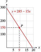
Next we find the \(x\)-coordinate of point \(P\) by drawing an imaginary line from \(P\) straight down to the \(x\)-axis. The \(x\)-coordinate of \(P\) is \(x = 9\text{.}\)
Thus, \(P\) is the point \((9,150)\text{,}\) and \(x = 9\) when \(y = 150\text{.}\) The solution of the equation \(150 = 285 - 15x\) is \(x = 9\text{.}\)
The relationship between an equation and its graph is an important one. For the previous example, make sure you understand that the following three statements are equivalent:
The point \((9, 150)\) lies on the graph of \(~y = 285 - 15x\text{.}\)
Consider again the graph of \(~y = 2x + 3~\text{,}\) shown at right. We saw that \(x = 2\) is the solution of the equation \(2x + 3 = 7\text{.}\) When we use \(x = 2\) as the input for the function \(f(x) = 2x + 3\text{,}\) the output is \(y = 7\text{.}\) Which input values for \(x\) produce output values greater than \(7\text{?}\)
You can see that \(x\)-values greater than \(2\) produce \(y\)-values greater than \(7\text{,}\) because points on the graph with \(x\)-values greater than \(2\) have \(y\)-values greater than \(7\text{.}\) Thus, the solutions of the inequality \(2x + 3 \gt 7\) are \(x\gt 2\text{.}\) You can verify this result by solving the inequality algebraically.
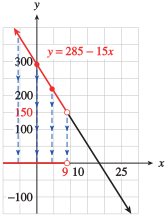
We begin by locating the point \(P\) on the graph for which \(y = 150\text{.}\) Its \(x\)-coordinate is \(x = 9\text{.}\) Now, because \(~y = 285 - 15x~\) for points on the graph, the inequality
So we are looking for points on the graph with \(y\)-coordinate greater than \(150\text{.}\) These points are shown in red on the graph. The \(x\)-coordinates of these points are the \(x\)-values that satisfy the inequality. From the graph, we see that the solutions are \(~x \lt 9\text{.}\)
You are using a graph of \(~f(x)=48-3.5x~\) to solve the inequality \(~48-3.5x \gt -15~\text{.}\) You find that \(~f(18)=-15\text{.}\) What is the solution to the inequality?
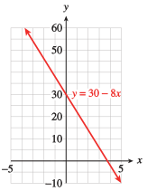
As we found in the previous Checkpoint, the point on \(y=30-8x\) where \(y=50 \) occurs when \(x=-2.5 \text{.}\) The \(y \)-coordinates are smaller as we move to the right on the graph, that is, for the points where \(x\ge -2.5 \text{.}\)
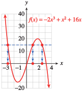
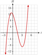
If we sketch in the horizontal line \(y = 15\text{,}\) we can see that there are three points on the graph of \(f\) that have \(y\)-coordinate \(15\text{,}\) as shown below. The \(x\)-coordinates of these points are the solutions of the equation.
From the graph, we see that the solutions are \(x = -3\text{,}\)\(x = 1\text{,}\) and approximately \(x = 2.5\text{.}\) We can verify each solution algebraically.
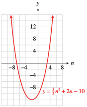
We look for points on the graph that have \(y\)-coordinate \(6\text{.}\) The \(n\)-coordinates of those two points are the solutions, \(n = -8\) and \(n = 4\text{.}\) To verify the solutions we evaluate the function at \(n = -8\) and \(n = 4\) to find
and trace along the curve to the point \((2.4680851, 15.512401)\text{.}\) We are close to a solution, because the \(y\)-value is close to \(15\text{.}\) Try entering \(x\)-values close to \(2.4680851\text{,}\) for instance, \(x = 2.4\) and \(x = 2.5\text{,}\) to find a better approximation for the solution.
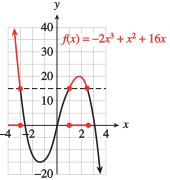
We first locate all points on the graph that have \(y\)-coordinates greater than or equal to \(15\text{.}\) The \(x\)-coordinates of these points are the solutions of the inequality.
The figure below shows those points in red, and their \(x\)-coordinates as intervals on the \(x\)-axis. The solutions are \(x \le -3\) and \(1\le x \le 2.5\text{,}\) or in interval notation, \((-\infty, -3] \cup [1, 2.5]\text{.}\) (See Appendix A.2 to review interval notation.)
In Practice 6 we found that \(\frac{1}{2}n^2 + 2n - 10 = 6 \) when \(n=-8\) and \(n=4\text{.}\) Looking at the graph, we see that points with \(y\)-coordinates less than 6 make up the lower portion of the parabola. They have \(x\)-coordinates between \(n=-8\) and \(n=4\text{.}\) Thus, the solutions are \(~ -8 \lt n \lt 4 \text{,}\) or in interval notation, \(~(-8,4)\)
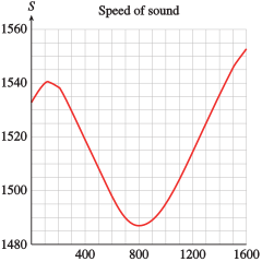
The graph shows the speed of sound in the ocean as a function of depth, \(S = f (d)\text{.}\) The speed of sound is affected both by increasing water pressure and by dropping temperature. (Source: Scientific American)
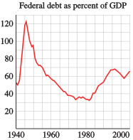
The graph shows the federal debt as a percentage of the gross domestic product (GDP), as a function of time, \(D = f (t)\text{.}\) (Source: Office of Management and Budget)
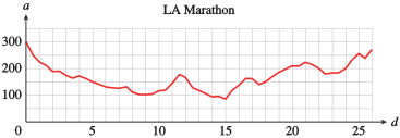
The graph shows the elevation (feet) of the 2005 Los Angeles Marathon course as a function of the distance (miles) into the race, \(a = f (d)\text{.}\) (Source: Los Angeles Times, March 3, 2005)
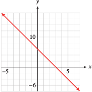
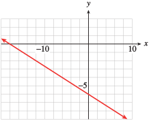
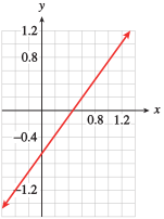
In Problems 23 and 24, use the graph to solve the equation or inequality, and then solve algebraically. (To review solving linear inequalities algebraically, see Algebra Skills Refresher A.2.)
For Problems 41–44, graph the equation with the ZInteger setting. (Press ZOOM\(6\text{,}\)then ZOOM\(8\)ENTER.) Use the graph to answer each question. Use the equation to verify your answers.
For Problems 45–48, graph the equation with the ZInteger setting. Use the graph to solve each equation or inequality. Check your solutions algebraically.
Press Y= and enter \(Y_2 = 10\text{.}\) Press GRAPH, and you should see the horizontal line \(y = 10\) superimposed on your previous graph. How many solutions does the equation
Press Y= and enter \(Y_2 = -5\text{.}\) Press GRAPH, and you should see the horizontal line \(y = -5\) superimposed on your previous graph. How many solutions does the equation