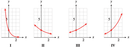
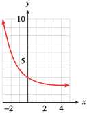
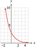
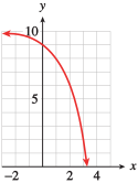
We do not allow \(b\) to be negative, because if \(b \lt 0\text{,}\) then \(b^x\) is not a real number for some values of \(x\text{.}\) For example, if \(b = -4\) and \(~f(x) = (-4)^x\text{,}\) then \(~f(1/2) = (-4)^{1/2}~\) is an imaginary number.
We also exclude \(b = 1\) as a base because \(1^x = 1\) for all values of \(x\text{;}\) hence the function \(~f(x) = 1^x\) is actually the constant function \(~f(x) = 1\text{.}\)
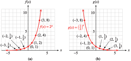
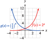
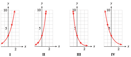
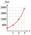
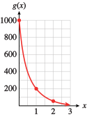
The graphs of exponential functions have two characteristic shapes, depending on whether the base, \(b\text{,}\) is greater than \(1\) or less than \(1\text{.}\) As typical examples, consider the graphs of \(f (x) = 2^x\) and \(g(x) =\left(\dfrac{1}{2}\right)^x\) shown below. Some values for \(f\) and \(g\) are recorded in the tables.
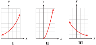
Notice that \(~f(x) = 2^x~\) is an increasing function and \(~g(x) = \left(\dfrac{1}{2}\right)^x~\) is a decreasing function. Both are concave up. In general, exponential functions have the following properties.
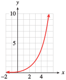
In the table for \(f(x)\text{,}\) you can see that as the \(x\)-values decrease toward negative infinity, the corresponding \(y\)-values decrease toward zero. As a result, the graph of \(f\) decreases toward the \(x\)-axis as we move to the left. Thus, the negative \(x\)-axis is a horizontal asymptote for exponential functions with \(b \gt 1\text{,}\) as shown in figure (a).
For exponential functions with \(0 \lt b \lt 1\text{,}\) the positive \(x\)-axis is an asymptote, as illustrated in figure (b). (See Section 2.2 to review asymptotes.)
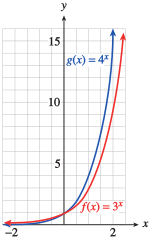
In Example 4.28, we compare two increasing exponential functions. The larger the value of the base, \(b\text{,}\) the faster the function grows. In this example, both functions have \(a = 1\text{.}\)
Then we plot the points for each function and connect them with smooth curves. For positive \(x\)-values, \(g(x)\) is always larger than \(f(x)\text{,}\) and is increasing more rapidly. In the figure, we can see that \(g(x) = 4^x\) climbs more rapidly than \(f(x) = 3^x\text{.}\) Both graphs cross the \(y\)-axis at (0, 1).
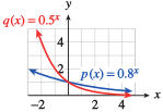
For decreasing exponential functions, those with bases between \(0\) and \(1\text{,}\) the smaller the base, the more steeply the graph decreases. For example, compare the graphs of \(~p(x) = 0.8^x~\) and \(~q(x) = 0.5^x~\) shown in the figure at right.
SubsectionTransformations of Exponential Functions
In Chapter 2, we considered transformations of the basic graphs. For instance, the graphs of the functions \(y = x^2 - 4\) and \(y = (x - 4)^2\) are shifts of the basic parabola, \(y = x^2\text{.}\) In a similar way, we can shift or stretch the graph of an exponential function while the basic shape is preserved.
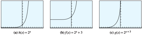
The graph of \(f(x) = 2^x + 3\text{,}\) shown in figure (b), has the same basic shape as that of \(h(x) = 2^x\text{,}\) but it has a horizontal asymptote at \(y = 3\) instead of at \(y = 0\) (the \(x\)-axis). In fact, \(f(x) = h(x) + 3\text{,}\) so the graph of \(f\) is a vertical translation of the graph of \(h\) by \(3\) units. If every point on the graph of \(h(x) = 2^x\) is moved \(3\) units upward, the result is the graph of \(f (x) = 2^x + 3\text{.}\)
First note that \(g(x) = 2^x+3 = h(x + 3)\text{.}\) In fact, the graph of \(g(x) = 2^{x+3}\) shown in figure (c) has the same basic shape as \(h(x) = 2^x\) but has been translated \(3\) units to the left.
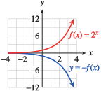
What about reflections? Recall that the graph of \(y = -f (x)\) is the reflection about the \(x\)-axis of the graph of \(y = f(x)\text{.}\) The graphs of \(y = 2^x\) and \(y = -2^x\) are shown at left below.
You may have also noticed a relationship between the graphs of \(~f(x) = 2^x~\) and \(~g(x) = \left(\dfrac{1}{2}\right)^x\text{,}\) which are shown at right above. The graph of \(g\) is the reflection of the graph of \(f\) about the \(y\)-axis. We can see why this is true by writing the formula for \(g(x)\) in another way:
We see that \(g(x)\) is the same function as \(f(-x)\text{.}\) Replacing \(x\) by \(-x\) in the formula for a function switches every point \((p,q)\) on the graph with the point \((-p,q)\) and thus reflects the graph about the \(y\)-axis.
SubsectionComparing Exponential and Power Functions
Exponential functions are not the same as the power functions we studied in Chapter 3. Although both involve expressions with exponents, it is the location of the variable that makes the difference.
The scaling exponent for \(h(x)\) is \(3\text{,}\) so that when \(x\) doubles, say, from \(1\) to \(2\text{,}\) the output is multiplied by \(2^3\text{,}\) or \(8\text{.}\)
On the other hand, we can tell that \(f\) is exponential because its values increase by a factor of \(3\) for each unit increase in \(x\text{.}\) (To see this, divide any function value by the previous one.)
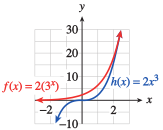
As you would expect, the graphs of the two functions are also quite different. For starters, note that the power function goes through the origin, while the exponential function has \(y\)-intercept \((0, 2)\)as shown at left below.
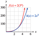
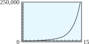
From the table, we see that \(h(3) = f(3) = 54\text{,}\) so the two graphs intersect at \(x = 3\text{.}\) (They also intersect at approximately \(x = 2.48\text{.}\)) However, if you compare the values of \(h(x) = 2x^3\) and \(f(x) = 2(3^x)\) for larger values of \(x\text{,}\) you will see that eventually the exponential function overtakes the power function, as shown at right above.
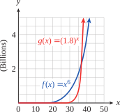
The relationship in Example 4.35 holds true for all increasing power and exponential functions: For large enough values of \(x\text{,}\) the exponential function will always be greater than the power function, regardless of the parameters in the functions. The figure at left shows the graphs of \(f(x) = x^6\) and \(g(x) = 1.8^x\text{.}\) At first, \(f(x) \gt g(x)\text{,}\) but at around \(x = 37\text{,}\)\(g(x)\) overtakes \(f(x)\text{,}\) and \(g(x) \gt f(x)\) for all \(x \gt 37\text{.}\)
In general, if two equivalent powers have the same base, then their exponents must be equal also, as long as the base is not \(0\) or \(\pm 1\text{.}\)
During the summer a population of fleas doubles in number every \(5\) days. If a population starts with \(10\) fleas, how long will it be before there are \(10,240\) fleas?
Let \(P\) represent the number of fleas present after \(t\) days. The original population of \(10\) is multiplied by a factor of \(2\) every \(5\) days, or
During an advertising campaign in a large city, the makers of Chip-O’s corn chips estimate that the number of people who have heard of Chip-O’s increases by a factor of \(8\) every 4 days.
If 100 people are given trial bags of Chip-O’s to start the campaign, write a function, \(N(t)\text{,}\) for the number of people who have heard of Chip-O’s after \(t\) days of advertising.
How many days should the makers run the campaign in order for Chip-O’s to be familiar to \(51,200\) people? Use algebraic methods to find your answer and verify on your graph.
Technology4.45Graphical Solution of Exponential Equations.
It is not always so easy to express both sides of the equation as powers of the same base. In the following sections, we will develop more general methods for finding exact solutions to exponential equations. But we can use a graphing utility to obtain approximate solutions.
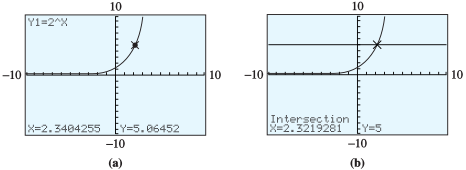
Enter \(Y_1 = 2\)^ X and use the standard graphing window (ZOOM 6) to obtain the graph shown in figure (a). We are looking for a point on this graph with \(y\)-coordinate \(5\text{.}\)
Using the TRACE feature, we see that the \(y\)-coordinates are too small when \(x \lt 2.1\) and too large when \(x \gt 2.4\text{.}\) The solution we want lies somewhere between \(x = 2.1\) and \(x = 2.4\text{,}\) but this approximation is not accurate enough.
To improve our approximation, we will use the intersect feature. Set \(Y_2 = 5\) and press GRAPH. The \(x\)-coordinate of the intersection point of the two graphs is the solution of the equation \(2^x = 5\) Activating the intersect command results in figure (b), and we see that, to the nearest hundredth, the solution is \(2.32\text{.}\)
We enter 2 ^ 2.32 ENTER to get \(4.993322196\text{.}\) This number is not equal to \(5\text{,}\) but it is close, so we believe that \(x = 2.32\) is a reasonable approximation to the solution of the equation \(2^x = 5\text{.}\)
For Problems 3–6, make a table of values and graph each pair of functions by hand on the domain \([-3, 3]\text{.}\) Describe the similarities and differences between the two graphs.
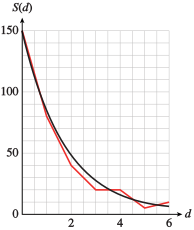
For several days after the Northridge earthquake on January 17, 1994, the area received a number of significant aftershocks. The red graph shows that the number of aftershocks decreased exponentially over time. The graph of the function \(S(d) = S_0b^d\text{,}\) shown in black, approximates the data. (Source: Los Angeles Times, June 27, 1995)
Find an approximation for the decay factor, \(b\text{,}\) by comparing two points on the graph. (Some of the points on the graph of \(S(d)\) are approximately \((1, 82)\text{,}\)\((2, 45)\text{,}\)\((3, 25)\text{,}\) and \((4, 14)\text{.}\))
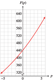
The frequency of a musical note depends on its pitch. The graph shows that the frequency increases exponentially. The function \(F(p) = F_0b^p\) gives the frequency as a function of the number of half-tones, \(p\text{,}\) above the starting point on the scale.
Find an approximation for the growth factor, \(b\text{,}\) by comparing two points on the graph. (Some of the points on the graph of \(F(p)\) are approximately \((1, 466)\text{,}\)\((2, 494)\text{,}\)\((3, 523)\text{,}\) and \((4, 554)\text{.}\))
The frequency doubles when you raise a note by one octave, which is equivalent to \(12\) half-tones. Use this information to find an exact value for \(b\text{.}\)
If the rancher does not act quickly, how long will it be until \(324\) head are affected? Use algebraic methods to find your answer, and verify it on your graph.
How long will it be before a \(\$700\) television set depreciates to \(\$343\text{?}\) Use algebraic methods to find your answer, and verify it on your graph.
How long will it be before a \(\$20,000\) mobile home depreciates to \(\$12,800\text{?}\) Use algebraic methods to find your answer, and verify it on your graph.
For Problems 47–50, decide whether the table could describe a linear function, a power function, an exponential function, or none of these. Find a formula for each linear, power, or exponential function.
For Problems 53–60, sketch the graph of each transformation of the given function, then write a formula and check your sketch with a graphing calculator. State the domain and range of each transformation, its intercept(s), and any asymptotes.
The function \(f (t)\) describes a volunteer’s heart rate during a treadmill test.
\begin{equation*}
f(t) =
\begin{cases}
100 \amp 0 \le t \lt 3\\
56t - 68 \amp 3 \le t \lt 4\\
186 - 500(0.5)^t \amp 4 \le t \lt 9\\
100 + 6.6(0.6)^{t-14} \amp 9\le t \lt 20
\end{cases}
\end{equation*}
The heart rate is given in beats per minute and \(t\) is in minutes. (See Section 2.2 to review functions defined piecewise.) (Source: Davis, Kimmet, and Autry, 1986)
The treadmill test began with walking at \(5.5\) kilometers per hour, then jogging, starting at \(12\) kilometers per hour and increasing to \(14\) kilometers per hour, and finished with a cool-down walking period. Identify each of these activities on the graph and describe the volunteer’s heart rate during each phase.
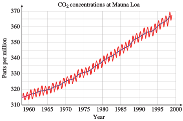
Carbon dioxide (\(\text{CO}_2\)) is called a greenhouse gas because it traps part of the Earth’s outgoing energy. Animals release \(\text{CO}_2\) into the atmosphere, and plants remove \(\text{CO}_2\) through photosynthesis. In modern times, deforestation and the burning of fossil fuels both contribute to \(\text{CO}_2\) levels. The figure shows atmospheric concentrations of \(\text{CO}_2\text{,}\) in parts per million, measured at the Mauna Loa Observatory in Hawaii.
The red curve shows annual oscillations in \(\text{CO}_2\) levels. Can you explain why \(\text{CO}_2\) levels vary throughout the year? Hint: Why would photosynthesis vary throughout the year?
The blue curve shows the average annual \(\text{CO}_2\) readings. By approximately how much does the \(\text{CO}_2\) level vary from its average value during the year?
In 1960, the average \(\text{CO}_2\) level was \(316.75\) parts per million, and the average level has been rising by \(0.4\%\) per year. If the level continues to rise at this rate, what \(\text{CO}_2\) readings can we expect in the year 2100?