When you buy a house, your monthly mortgage payment is a function of the size of the loan. The table shows mortgage payments on \(30\)-year loans of various sizes at \(6\)% interest.
However, when you are shopping for a house, you may think of the mortgage payment as the input variable: If you can afford a certain monthly mortgage payment, how large a loan can you finance? Now the mortgage payment is the input value, and the loan amount is the output. By interchanging the inputs and outputs, we define a new function, \(L = g(M)\text{,}\) shown below.
This new function gives the same information as the original function, \(f\text{,}\) but from a different point of view. We call the function \(g\) the inverse function for \(f\text{.}\)
The elements of the range of \(f\) are used as the input values for \(g\text{,}\) and the output values of \(g\) are the corresponding domain elements of \(f\text{.}\) For example, from the tables you can verify that \(f (200,000) = 1199.10\text{,}\) and \(g(1199.10) = 200,000\text{.}\) In fact, this property defines the inverse function.
We know that \(g(5) = -3\) because \(f(-3) = 5\text{,}\) and \(g(0) = 5\) because \(f(5) = 0\text{.}\) Tables may be helpful in visualizing the two functions, as shown below.
For the function \(f\text{,}\) the input variable is \(x\) and the output variable is \(y\text{.}\) For the inverse function \(g\text{,}\) the roles of the variables are interchanged: \(y\) is now the input and \(x\) is the output.
SubsectionFinding a Formula for the Inverse Function
If a function is given by a table of values, we can interchange the columns (or rows) of the table to obtain the inverse function. Swapping the columns works because we are really interchanging the input and output variables. If a function is defined by an equation, we can find a formula for its inverse function in the same way: Interchange the roles of the variables in the equation so that the old output variable becomes the new input variable.
The function \(H = f(t) = 6 + 2t\) gives the height of corn seedlings, in inches, \(t\) days after they are planted. Find a formula for the inverse function and explain its meaning in this context.
To make a table for \(g\text{,}\) we could choose values for \(H\) and evaluate \(~\dfrac{H-6}{2}\text{,}\) but because \(g\) is the inverse function for \(f\text{,}\) we can simply interchange the columns in our table for \(f\text{,}\) as shown at right above.
Note once again that the two tables show the same relationship between \(t\) and \(H\text{,}\) but the roles of input and output have been interchanged. The function \(f\) tells us the height of the seedlings after \(t\) days, and \(g\) tells us how long it will take the seedlings to grow to height \(H\text{.}\)
Carol can burn 600 calories per hour bicycling and 400 calories per hour swimming. She would like to lose 5 pounds, which is equivalent to 16,000 calories.
Write an equation relating the number of hours of cycling, \(x\text{,}\) and the number of hours swimming, \(y\text{,}\) that Carol must spend to lose 5 pounds.
If the inverse of a function \(f\) is also a function, we denote the inverse by the symbol \(f^{-1}\text{,}\) read "\(f\) inverse." This notation makes it clear that the two functions are related in a special way. For example, the function \(~f(t) = 6 + 2t\) in Example 5.4 has inverse function \(~f^{-1}(H) = \dfrac{H -6}{2}\text{.}\)
Although the same symbol, \(^{-1}\text{,}\) is used for both reciprocals and inverse functions, the two notions are not equivalent. That is, the inverse of a given function is usually not the same as the reciprocal of that function. In Example 5.4, note that \(f^{-1}(y)\) is not the same as the reciprocal of \(f (y)\text{,}\) because
are equivalent; they convey the same information. This fact is a restatement of our earlier observation about inverse functions, this time using inverse function notation.
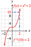
We can use a graph of a function \(y = f(x)\) to find values of the inverse function \(x = f^{-1}(y)\text{.}\) The figure below shows the graph of \(f(x) = x^3 + 2\text{.}\)
You already know how to evaluate a function from its graph: We start with the horizontal axis. For instance, to evaluate \(f(-2)\text{,}\) we find \(-2\) on the \(x\)-axis, move vertically to the point on the graph with \(x = -2\text{,}\) in this case \((-2, -6)\text{,}\) and read the \(y\)-coordinate of the point. We see that \(f(-2) = -6\text{.}\)
To evaluate the inverse function, we start with the vertical axis. For example, to find \(f^{-1}(10)\text{,}\) we find \(10\) on the vertical axis and move horizontally to the point on the graph with \(y = 10\text{.}\) In this case, the point is \((2, 10)\text{,}\) so \(f^{-1}(10) = 2\text{.}\)
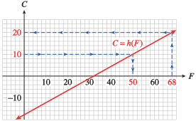
The function \(C = h(F)\) gives Celsius temperature as a function of Fahrenheit temperature. The graph of the function is shown below. Use the graph to evaluate \(h(68)\) and \(h^{-1}(10)\text{,}\) and then explain their meaning in this context.
To evaluate \(h(68)\text{,}\) we find the input \(F = 68\) on the horizontal axis, then find the point on the graph with \(F = 68\) and read its vertical coordinate. We see that the point \((68, 20)\) lies on the graph, so \(h(68) = 20\text{.}\) When the Fahrenheit temperature is \(68\degree\text{,}\) the Celsius temperature is \(20\degree\text{.}\)
The inverse function reverses the roles of input and output. Because \(C = h(F)\text{,}\)\(F = h^{-1}(C)\text{,}\) so the inverse function gives us the Fahrenheit temperature if we know the Celsius temperature. In particular, \(h^{-1}(10)\) is the Fahrenheit temperature when the Celsius temperature is \(10\degree\text{.}\)
To use the graph of \(h\) to find values of \(h^{-1}\text{,}\) we start with the vertical axis and find the point on the graph with \(C = 10\text{.}\) This point is \((50, 10)\text{,}\) so \(F = 50\) when \(C = 10\text{,}\) or \(h^{-1}(10) = 50\text{.}\) When the Celsius temperature is \(10\degree\text{,}\) the Fahrenheit temperature is \(50\degree\text{.}\)
Write two equations, one using \(h\) and one using \(h^{-1}\text{,}\) stating the Fahrenheit temperature when the Celsius temperature is \(0^\circ\text{.}\)
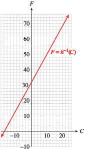
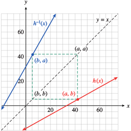
In Example 5.13, we used a graph of \(h\) to read values of \(h^{-1}\text{.}\) But we can also plot the graph of \(h^{-1}\) itself. Because \(C\) is the input variable for \(h^{-1}\text{,}\) we plot \(C\) on the horizontal axis and \(F\) on the vertical axis. To find some points on the graph of \(h^{-1}\text{,}\) we interchange the coordinates of points on the graph of \(h\text{.}\) The graph of \(h^{-1}\) is shown at right.
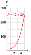
The Park Service introduced a flock of \(12\) endangered pheasant into a wildlife preserve. After \(t\) years, the population of the flock was given by
\begin{equation*}
P = f(t) = 12 + 2t^3
\end{equation*}
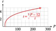
We solve \(~P = 12 + 2t^3\) for \(t\) in terms of \(P\text{.}\)
\begin{equation*}
\begin{aligned}[t]
2t^3 \amp = P - 12\amp\amp \blert{\text{Substract 12 from both sides.}}\\
t^3 \amp = \frac{P - 12}{2}\amp\amp \blert{\text{Divide both sides by 2.}}\\
t \amp = \sqrt[3]{\frac{P - 12}{2}}\amp\amp \blert{\text{Take cube roots.}}
\end{aligned}
\end{equation*}
The inverse function is \(~t = f^{-1}(P) =\sqrt[3]{\dfrac{P - 12}{2}}\text{.}\) It tells us the number of years it takes for the pheasant population to grow to size \(P\text{.}\)
The formula \(~T = f(L) = 2\pi \sqrt{\dfrac{L}{32}}\) gives the period in seconds, \(T\text{,}\) of a pendulum as a function of its length in feet, \(L\text{.}\)
We can always find the inverse of a function simply by interchanging the input and output variables. In the preceding examples, interchanging the variables created a new function. However, the inverse of a function does not always turn out to be a function itself.
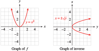
For example, to find the inverse of \(~y = f(x) = x^2\text{,}\) we solve for \(x\) to get \(~x = \pm\sqrt{y}\text{.}\) When we regard \(y\) as the input and \(x\) as the output, the relationship does not describe a function. The graphs of \(f\) and its inverse are shown below. (Note that for the graph of the inverse, we plot \(y\) on the horizontal axis and \(x\) on the vertical axis.) Because the graph of the inverse does not pass the vertical line test, it is not a function.
For many applications, it is important to know whether or not the inverse of \(f\) is a function. This can be determined from the graph of \(f\text{.}\) When we interchange the roles of the input and output variables, horizontal lines of the form \(y = k\) become vertical lines.
Thus, if the graph of the inverse is going to pass the vertical line test, the graph of the original function must pass the horizontal line test, namely, that no horizontal line should intersect the graph in more than one point.
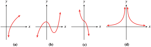
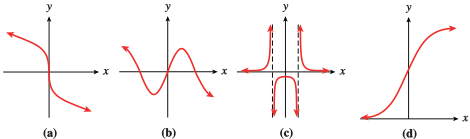
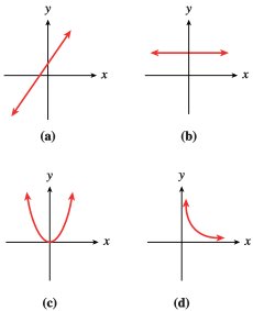
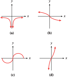
In each case, we apply the horizontal line test to determine whether the inverse is a function. Because no horizontal line intersects their graphs more than once, the functions pictured in figures (a) and (c) have inverses that are also functions. The functions in figures (b) and (d) do not have inverses that are functions.
A function that passes the horizontal line test is called one-to-one, because each input has only one output and each output has only one input. A one-to-one function passes the horizontal line test as well as the vertical line test. With this terminology, we can state the following theorem.
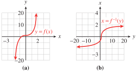
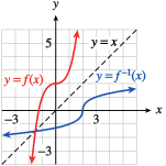
A function may have an inverse function even if we cannot find its formula. The function \(~f(x) = x^5 + x + 1~\) shown in figure (a) is one-to-one, so it has an inverse function. We can even graph the inverse function, as shown in figure (b), by interchanging the coordinates of points on the graph of \(f\text{.}\)
However, we cannot find a formula for the inverse function because we cannot solve the equation \(~y = x^5 + x + 1~\) for \(x\) in terms of \(y\text{.}\)
SubsectionMathematical Properties of the Inverse Function
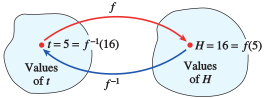
The inverse function \(f^{-1}\) undoes the effect of the function \(f\text{.}\) In Example 5.4, the function \(~f(t) = 6 + 2t~\) multiplies the input by \(2\) and then adds \(6\) to the result. The inverse function \(f^{-1}(H) = \dfrac{H -6}{2}\) undoes those operations in reverse order: It subtracts \(6\) from the input and then divides the result by \(2\text{.}\)
If we apply the function \(f\) to a given input value and then apply the function \(f^{-1}\) to the output from \(f\text{,}\) the end result will be the original input value. For example, if we choose \(t = \alert{5}\) as an input value, we find that
\begin{equation*}
\begin{aligned}[t]
f(\alert{5})\amp= 6 + 2(\alert{5})
= \blert{16}\amp\amp \blert{\text{ Multiply by 2, then add 6.}}\\
\text{and } f^{-1}(\blert{16}) \amp = \frac{\blert{16} - 6}{2}
= \alert{5}\amp\amp \blert{\text{Subtract 6, then divide by 2.}}
\end{aligned}
\end{equation*}
Example 5.23 illustrates the fact that if \(f^{-1}\) is the inverse function for \(f\text{,}\) then \(f\) is also the inverse function for \(f^{-1}\text{.}\)
So far we have been careful to keep track of the input and output variables when we work with inverse functions. This is important when we are dealing with applications; the names of the variables are usually chosen because they have a meaning in the context of the application, and it would be confusing to change them.
However, we can also study inverse functions purely as mathematical objects. There is a relationship between the graph of a function and the graph of its inverse that is easier to see if we plot them both on the same set of axes.
A graph does not change if we change the names of the variables, so we can let \(x\) represent the input for both functions, and let \(y\) represent the output. Consider the function \(C = h(F)\) from Example 5.13, and its inverse function, \(F = h^{-1}(C)\text{.}\) The formulas for these functions are
\begin{equation*}
\begin{aligned}[t]
C \amp = h(F) = \frac{5}{9}(F - 32)\\
F \amp = h^{-1}(C) = 32 + \frac{9}{5}C
\end{aligned}
\end{equation*}
But their graphs are the same if we write them as
\begin{equation*}
\begin{aligned}[t]
y \amp = h(x) =\frac{5}{9}(x - 32)\\
y \amp= h^{-1}(x) = 32 + \frac{9}{5}x
\end{aligned}
\end{equation*}
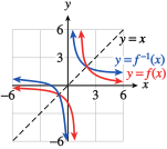
Now, for every point \((a, b)\) on the graph of \(f\text{,}\) the point \((b, a)\) is on the graph of the inverse function. Observe that the points \((a, b)\) and \((b, a)\) are always located symmetrically across the line \(y=x\text{.}\) The graphs are symmetric about the line \(y=x\), which means that if we were to place a mirror along the line \(y=x\text{,}\) each graph would be the reflection of the other.
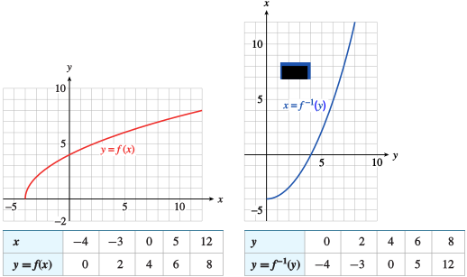
The graph of \(f\) has the same shape as the graph of \(y = \sqrt{x}\text{,}\) shifted \(4\) units to the left and stretched vertically by a factor of \(2\text{.}\) The figure at left below shows the graph of \(f\text{,}\) along with a table of values. By interchanging the rows of the table, we obtain points on the graph of the inverse function, shown at right.
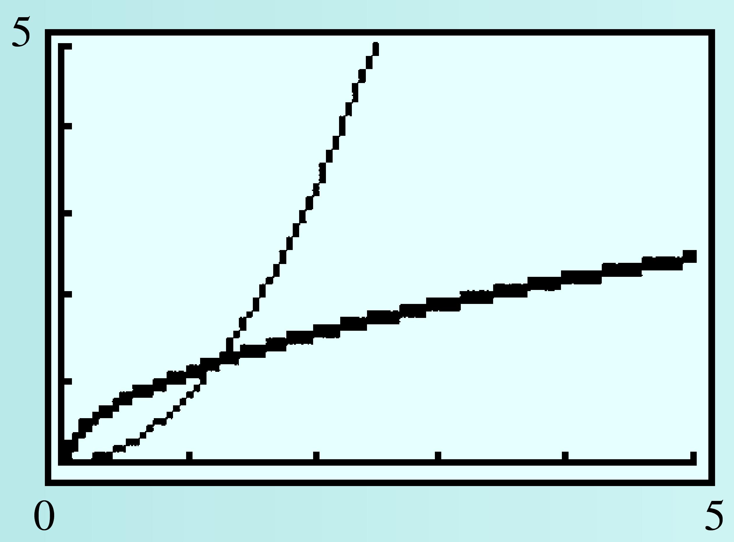
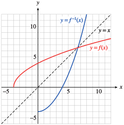
If we use \(x\) as the input variable for both functions, and \(y\) as the output, we can graph \(f\) and \(f^{-1}\) on the same grid, as shown at right. The two graphs are symmetric about the line \(y = x\text{.}\)
Graph the function \(~f(x) = x^3 + 2~\) and its inverse \(~f^{-1}(x) = \sqrt[3]{x - 2}~\) on the same set of axes, along with the line \(y = x\text{.}\)
When we interchange the input and output variables to obtain the inverse function, we interchange the domain and range of the function. For the functions graphed in Example 5.26, you can see that
To find the inverse function, we solve for \(x\text{.}\) Take the reciprocal of both sides of the equation.
\begin{equation*}
\begin{aligned}[t]
\dfrac{1}{y} \amp= x + 3\amp\amp \blert{\text{Subtract 3 from both sides.}}\\
x \amp = \dfrac{1}{y}- 3
\end{aligned}
\end{equation*}
The inverse function is \(~x = f^{-1}(y) = \dfrac{1}{y}- 3\text{,}\) or, using \(x\) for the input variable, \(~f^{-1}(x) = \dfrac{1}{x}- 3\text{.}\) The graph of \(f^{-1}\) looks like the graph of \(y = \dfrac{1}{x}\text{,}\) shifted down \(3\) units, as shown below.
Because \(f\) is undefined at \(x = -3\text{,}\) the domain of \(f\) is all real numbers except \(-3\text{.}\) The graph has a horizontal asymptote at \(y = 0\text{,}\) so the range is all real numbers except \(0\text{.}\)
The inverse function \(~f^{-1}(x) = \dfrac{1}{x}- 3~\) is undefined at \(x = 0\text{,}\) so its domain is all real numbers except \(0\text{.}\) The graph of \(f^{-1}\) has a horizontal asymptote at \(y = -3\text{,}\) so its range is all real numbers except \(-3\text{.}\)
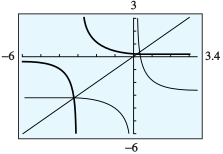
Graph the function \(~f(x) = \dfrac{2}{x -1}\) and its inverse function, \(f^{-1}\) (which you found above in Practice 7, on the same set of axes, along with the line \(y = x\text{.}\)
Domain of \(f\text{:}\) all real numbers except \(1\text{,}\) Range of \(f\text{:}\) all real numbers except \(0\text{,}\) Domain of \(f^{-1}\text{:}\) all real numbers except \(0\text{,}\) Range of \(f^{-1}\text{:}\) all real numbers except \(1\)
If a function is defined by a formula in the form \(y = f (x)\text{,}\) we can find a formula for its inverse function by solving the equation for \(x\) to get \(x = f^{-1}(y)\text{.}\)
The inverse function \(f^{-1}\) undoes the effect of the function \(f\text{,}\) that is, if we apply the inverse function to the output of \(f\text{,}\) we return to the original input value.
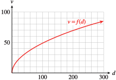
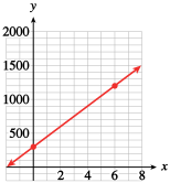
An insurance investigator measures the length, \(d\text{,}\) of the skid marks at an accident scene, in feet. The graph shows the function \(v = f (d)\text{,}\) which gives the velocity, \(v\) (mph), at which a car was traveling when it hit the brakes.
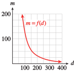
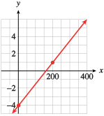
The weight, \(m\text{,}\) of a missile launched from a catapult is a function of the distance, \(d\text{,}\) to the target. The graph shows the function \(m = f (d)\text{,}\) where \(d\) is in meters and \(m\) is in kilograms.
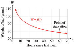
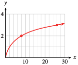
After eating, the weight of a vampire bat drops steadily until its next meal. The graph shows the function \(W = f (t)\text{,}\) which gives the weight, \(W\text{,}\) of the bat in grams \(t\) hours since its last meal.
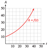
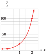
The amount of money, \(A\text{,}\) in an interest-bearing savings account is a function of the number of years, \(t\text{,}\) it remains in the account. The graph shows \(A = f (t)\text{,}\) where \(A\) is in thousands of dollars.
The function \(I = g(r ) = (1 + r )^5 - 1\) gives the interest, \(I\text{,}\) that a dollar earns in \(5\) years in terms of the interest rate, \(r\text{.}\)
Evaluate \(g(0.05)\) and explain what it tells us about the interest.
If you are flying in an airplane at an altitude of \(h\) miles, on a clear day you can see a distance of \(d\) miles to the horizon, where \(d = f (h) = \sqrt{7920h}\text{.}\)
Evaluate \(f(0.5)\) and explain what it tells us about the horizon.
A moving ship creates waves that impede its own speed. The function \(v = f (L) = 1.3\sqrt{L}\) gives the ship’s maximum speed in knots in terms of its length, \(L\text{,}\) in feet.
Evaluate \(f(400)\) and explain what it tells us about the ship’s speed.
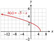
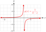
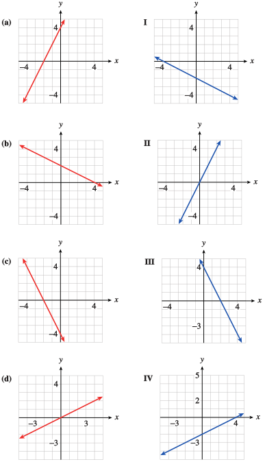
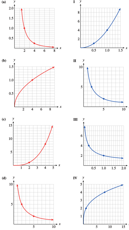
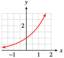
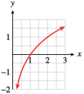
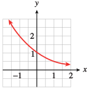
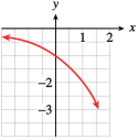
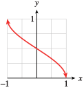
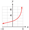
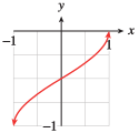
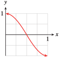
For Problems 45 and 46, use the graph of \(f\) to match the other graphs with the appropriate function. (Hint: Look at the coordinates of some specific points.)