The models we have explored so far are linear models; their graphs are straight lines. In this chapter, we investigate problems where the graph may change from increeasing to decreasing, or vice versa. The simplest sort of function that models this behavior is a quadratic function, one that involves the square of the variable.
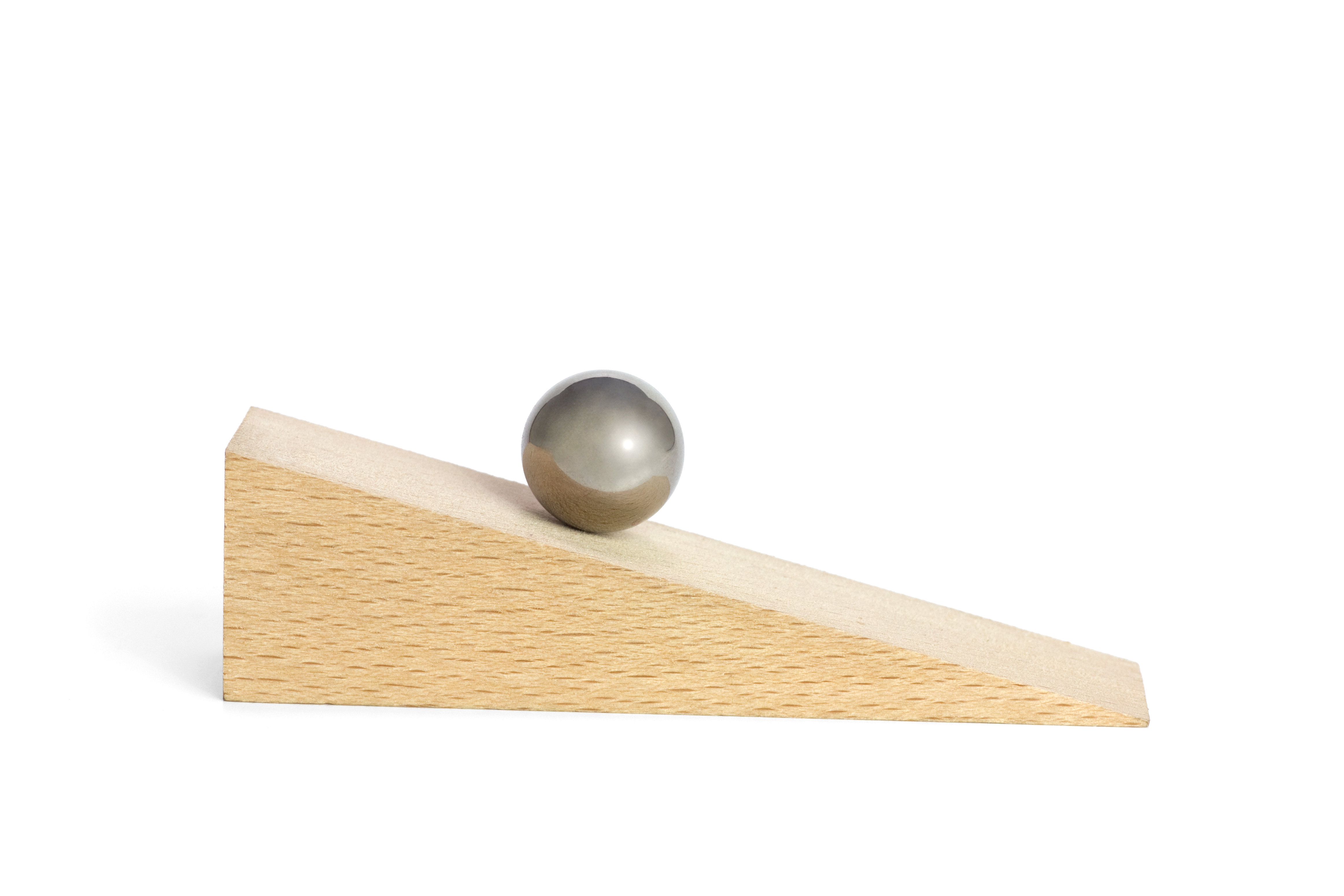
Around 1600, Galileo began to study the motion of falling objects. He used a ball rolling down an inclined plane or ramp to slow down the motion, but he had no accurate way to measure time; clocks had not been invented yet. So he used water running into a jar to mark equal time intervals.
After many trials, Galileo found that the ball traveled 1 unit of distance down the plane in the first time interval, 3 units in the second time interval, 5 units in the third time interval, and so on, as shown in the figure, with the distances increasing through odd units of distance as time went on.
The total distance traveled by the ball can be modeled by the equation, \(d = kt^2\text{,}\) where \(k\) is a constant. Galileo found that this relationship holds no matter how steep he made the ramp. If we plot the height of the ball (rather than the distance traveled) versus time, we obtain a portion of the graph of a quadratic equation.
Suppose you drop a small object from a height and let it fall under the influence of gravity. Does it fall at the same speed throughout its descent? The diagram shows a sequence of photographs of a steel ball falling onto a table. The photographs were taken using a stroboscopic flash at intervals of 0.05 second, and a scale on the left side shows the height of the ball, in feet, at each interval.
Complete the table showing the height of the ball at each 0.05-second interval. Measure the height at the bottom of the ball in each image. The first photo was taken at time \(t=0\text{.}\)
What was the change in the ball’s height during the first quarter second, from \(t=0\) to \(t=0.25\) ? What was the change in the ball’s height from \(t=0.25\) to \(t=0.50\) ?
Add to your graph a line segment connecting the points at \(t=0\) and \(t=0.25\text{,}\) and a second line segment connecting the points at \(t=0.25\) and \(t=0.50\text{.}\) Compute the slope of each line segment.