Warm Up
1.1.3.1.
Answer.
-
\(\displaystyle 5.5\)
-
\(\displaystyle 12\)
1.1.3.3.
Answer.
\(I=200+0.09 S\)
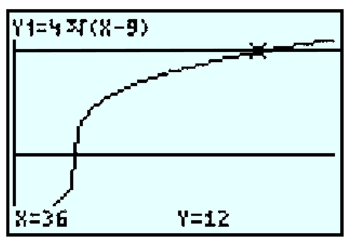
| \(t\) (days) | \(0\) | \(5\) | \(10\) | \(15\) | \(20\) |
| \(h\) (inches) | 6 | 16 | 26 | 36 | 46 |

| Altitude (1000 ft) | \(0\) | \(1\) | \(2\) | \(3\) | \(4\) | \(5\) |
| Boiling point (\(\degree\)F) | \(212\) | \(210\) | \(208\) | \(206\) | \(204\) | \(202\) |


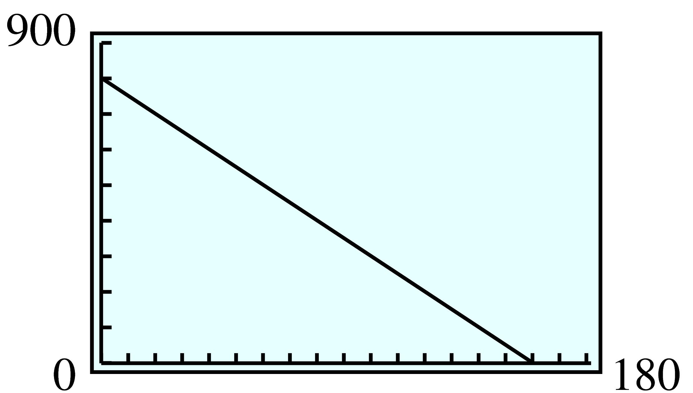
| \(~ t ~\) | \(0\) | \(5\) | \(10\) | \(15\) | \(20\) |
| \(~ h ~\) | \(-400\) | \(-300\) | \(-200\) | \(-100\) | \(0\) |


| \(x\) | \(-1\) | \(~0~\) | \(~2~\) | \(~3~\) | \(~4~\) |
| \(y\) | \(10\) | \(8\) | \(4\) | \(2\) | \(0\) |


| \(h\) | \(8\) | \(20\) |
| \(C\) | \(645\) | \(1425\) |
| \(C\) | \(15\) | \(-5\) |
| \(F\) | \(59\) | \(23\) |


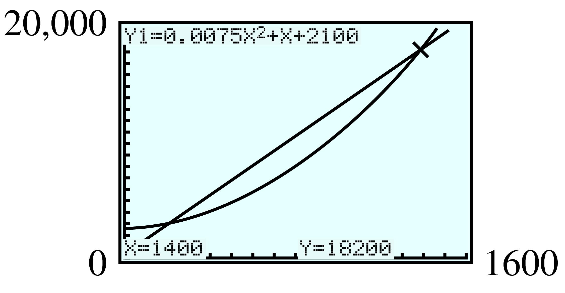
| \(n\) | \(100\) | \(500\) | \(800\) | \(1200\) | \(1500\) |
| \(C\) | \(4000\) | \(12,000\) | \(18,000\) | \(26,000\) | \(32,000\) |

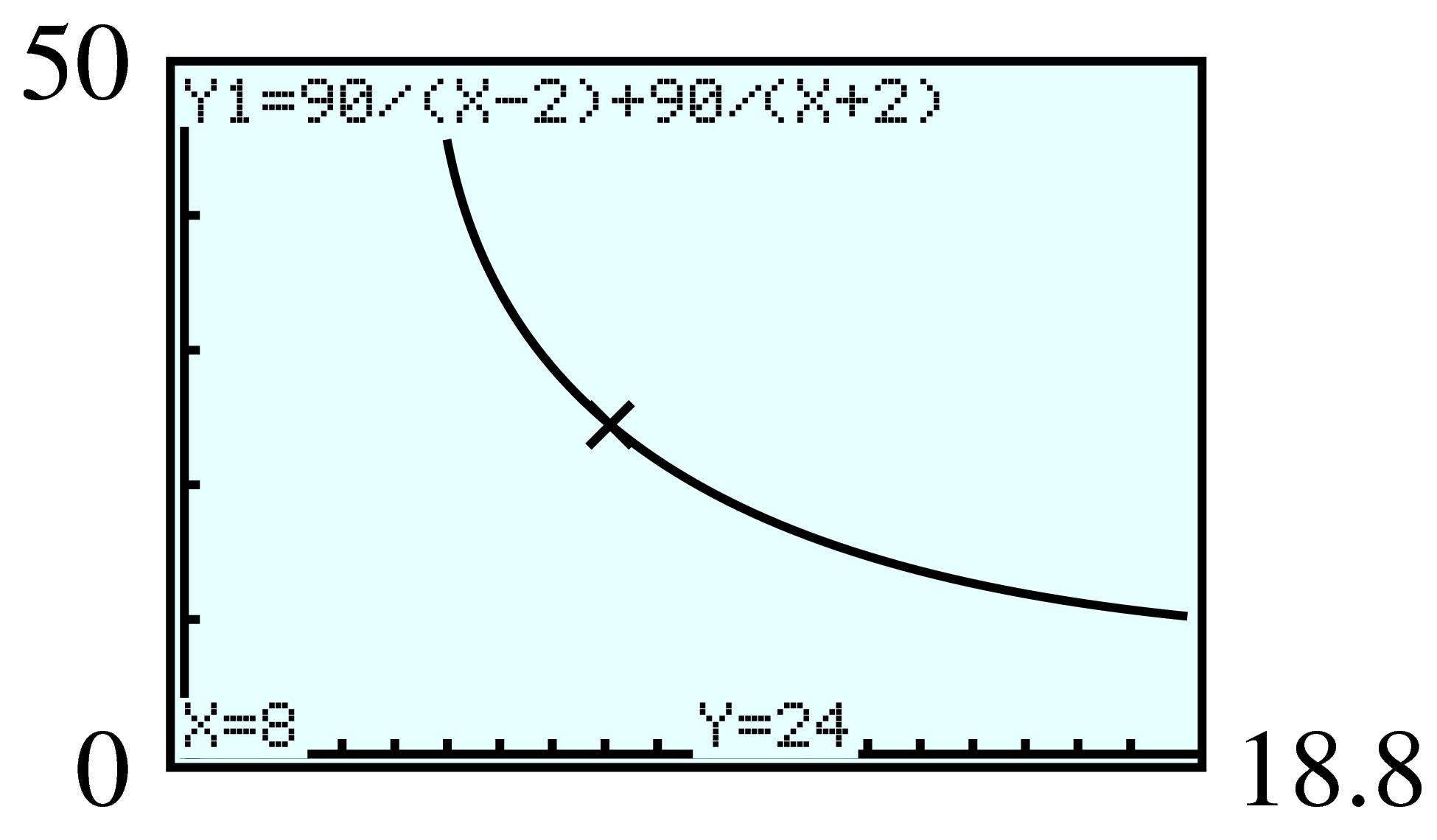
| \(t\) | \(~ 5 ~\) | \(~10~\) | \(~15~\) | \(~20~\) | \(~25~\) |
| \(R\) | \(1960\) | \(1820\) | \(1680\) | \(1540\) | \(1400\) |


| \(t\) | \(0\) | \(15\) |
| \(P\) | \(4800\) | \(6780\) |
| \(k\) | \(70\) | \(50\) |
| \(p\) | \(154\) | \(110\) |


| \(x\) | Sporthaus | Fitness First |
| 6 | 560 | 200 |
| 12 | 620 | 350 |
| 18 | 680 | 500 |
| 24 | 740 | 650 |
| 30 | 800 | 800 |
| 36 | 860 | 950 |
| 42 | 920 | 1100 |
| 48 | 980 | 1250 |


| Pounds | % silver | Amount of silver | |
| First alloy | \(x\) | \(0.45\) | \(0.45x\) |
| Second alloy | \(y\) | \(0.60\) | \(0.60y\) |
| Mixture | \(40\) | \(0.48\) | \(0.48(40)\) |
| Rani’s speed in still water: | \(x\) |
| Speed of the current: | \(y\) |
| Rate | Time | Distance | |
| Downstream | \(x+y\) | \(45\) | \(6000\) |
| Upstream | \(x-y\) | \(45\) | \(4800\) |
| Sports coupes | Wagons | Total | |
| Hours of riveting | 3 | 4 | 120 |
| Hours of welding | 4 | 5 | 155 |
| Principal | Interest rate | Interest | |
| Bonds | \(x\) | \(0.10\) | \(0.10x\) |
| Certificate | \(y\) | \(0.08\) | \(0.08y\) |
| Total | \(2000\) | —— | \(184\) |
| \(x\) | \(-2\) | \(5\) | \(6\) | \(8\) |
| \(y\) | \(12\) | \(5\) | \(4\) | \(2\) |


| \(~r~\) | \(0.02\) | \(0.04\) | \(0.06\) | \(0.08\) |
| \(~A~\) | \(1664.64\) | \(1730.56\) | \(1797.76\) | \(1866.24\) |


| \(t\) | \(0\) | \(0.25\) | \(0.5\) | \(0.75\) | \(1\) | \(0.25\) | \(1.5\) |
| \(h\) | \(-12\) | \(-5\) | \(0\) | \(3\) | \(4\) | \(3\) | \(0\) |


| \(~~~~\) | \(x \lt -4\) | \(-4 \lt x \lt 2\) | \(x \gt 2\) |
| \(Y_1\) | \(-\) | \(+\) | \(+\) |
| \(Y_2\) | \(-\) | \(-\) | \(+\) |
| \(Y_3\) | \(+\) | \(-\) | \(+\) |


| \(x\) | \(2\) | \(5\) | \(8\) | \(12\) | \(15\) |
| \(y\) | \(-0.6\) | \(1.5\) | \(2.4\) | \(3.6\) | \(4.5\) |
| \(\text{Price of item} \) | \(18\) | \(28\) | \(12\) |
| \(\text{Tax} \) | \(1.17\) | \(1.82\) | \(0.78\) |
| \(\text{Tax}/\text{Price} \) | \(\alert{0.065}\) | \(\alert{0.065}\) | \(\alert{0.065}\) |

| \(w\) | \(50\) | \(100\) | \(200\) | \(400\) |
| \(m\) | \(\alert{8.25}\) | \(\alert{16.5}\) | \(\alert{33}\) | \(\alert{66}\) |
| \(w\) | \(10\) | \(20\) | \(40\) | \(80\) |
| \(P\) | \(\alert{223} \) | \(\alert{1782} \) | \(\alert{14,259} \) | \(\alert{114,074} \) |
| \(x\) | \(4\) | \(8\) | \(20\) | \(30\) | \(40\) |
| \(y\) | \(30\) | \(15\) | \(6\) | \(4\) | \(3\) |
| \(\text{Width (feet)} \) | \(2\) | \(2.5\) | \(3\) |
| \(\text{Length (feet)} \) | \(12\) | \(9.6\) | \(8\) |
| \(\text{Length}\times \text{width} \) | \(\alert{24}\) | \(\alert{24}\) | \(\alert{24}\) |

| \(d\) | \(1\) | \(2\) | \(12\) | \(24\) |
| \(B\) | \(\alert{88} \) | \(\alert{44} \) | \(\alert{7.3} \) | \(\alert{3.7} \) |


| \(x\) | \(0\) | \(4\) | \(8\) | \(14\) | \(16\) | \(22\) |
| \(y\) | \(24\) | \(20\) | \(16\) | \(10\) | \(8\) | \(2\) |
| \(x\) | \(0\) | \(4\) | \(10\) | \(12\) | \(14\) | \(16\) |
| \(y\) | \(0\) | \(6\) | \(15\) | \(18\) | \(21\) | \(24\) |
| \(x\) | \(0\) | \(1\) | \(4\) | \(9\) | \(16\) | \(25\) |
| \(y\) | \(0\) | \(1\) | \(2\) | \(3\) | \(4\) | \(5\) |
| \(x\) | \(0.25\) | \(0.50\) | \(1.00\) | \(1.50\) | \(2.00\) | \(4.00\) |
| \(y\) | \(4.00\) | \(2.00\) | \(1.00\) | \(0.67\) | \(0.50\) | \(0.25\) |
| \(x\) | \(-3\) | \(-2\) | \(-1\) | \(0\) | \(1\) | \(2\) |
| \(y\) | \(5\) | \(0\) | \(-3\) | \(-4\) | \(-3\) | \(0\) |
| \(x\) | \(-3\) | \(-2\) | \(-1\) | \(0\) | \(1\) | \(4\) |
| \(y\) | \(0\) | \(5\) | \(8\) | \(9\) | \(8\) | \(-7\) |
| \(x\) | \(1\) | \(2\) | \(4.5\) | \(6.2\) | \(9.3\) |
| \(g(x)\) | \(1\) | \(0.125\) | \(0.011\) | \(0.0042\) | \(0.0012 \) |
| \(x\) | \(1.5\) | \(0.6\) | \(0.1\) | \(0.03\) | \(0.002\) |
| \(f(x)\) | \(0.30\) | \(4.63\) | \(1000\) | \(37,037\) | \(125 \times 10^6\) |
| \(L\) (feet) | \(200\) | \(400\) | \(600\) | \(800\) | \(1000\) |
| \(v_{\text{max}}\) (knots) | \(18.4\) | \(26\) | \(31.8\) | \(36.8\) | \(41.1\) |


| Element | Carbon | Potassium | Cobalt | Technetium | Radium |
| Mass number, \(A\) |
\(14\) | \(40\) | \(60\) | \(99\) | \(226\) |
| Radius, \(r\) (\(10^{-13}\) cm) |
\(3.1\) | \(4.4\) | \(5.1\) | \(6\) | \(7.9\) |

| \(x\) | \(0\) | \(1\) | \(2\) | \(3\) | \(4\) | \(5\) | \(6\) |
| \(f(x)\) | \(0\) | \(1\) | \(2.5\) | \(4.3\) | \(6.4\) | \(8.5\) | \(10.9\) |
| \(g(x)\) | \(0\) | \(1\) | \(2.8\) | \(5.2\) | \(8\) | \(11.2\) | \(14.7\) |

| \(t\) | \(5\) | \(10\) | \(15\) | \(20\) |
| \(I(t)\) | \(131\) | \(199\) | \(254\) | \(302\) |
| \(A\) | \(10\) | \(100\) | \(1000\) | \(5000\) | \(10,000\) |
| \(S\) | \(25 \) | \(42 \) | \(69 \) | \(98 \) | \(115 \) |


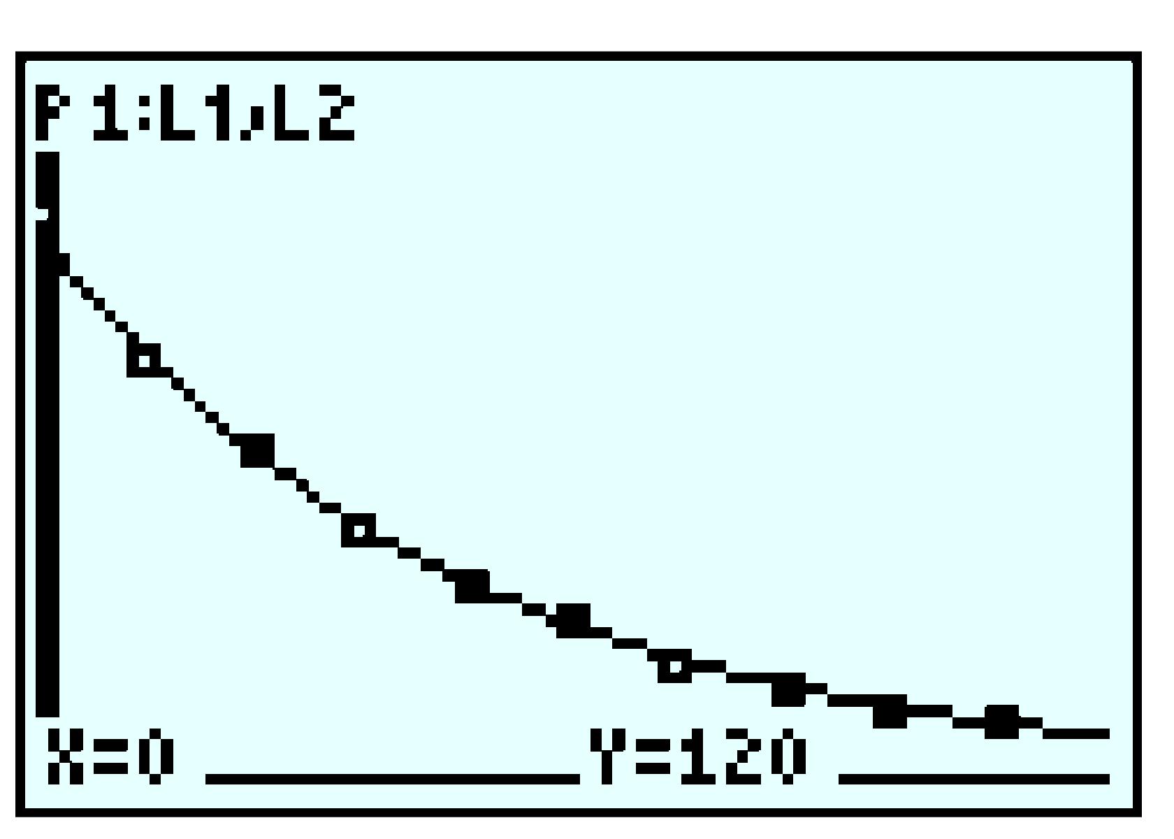
| \(x\) | \(y\) |
| \(-25\) | \(6.92\) |
| \(-20\) | \(6.71\) |
| \(-15\) | \(6.47\) |
| \(-10\) | \(6.15\) |
| \(-5\) | \(3.21\) |
| \(0\) | \(4\) |
| \(5\) | \(2.29\) |
| \(10\) | \(1.85\) |
| \(15\) | \(1.53\) |
| \(20\) | \(1.29\) |

| Planet | Density |
| Mercury | 5426 |
| Venus | 5244 |
| Earth | 5497 |
| Mars | 3909 |
| Jupiter | 1241 |
| Saturn | 620 |
| Uranus | 1238 |
| Neptune | 1615 |
| Pluto | 2355 |


| \(x\) | \(0\) | \(1\) | \(2\) | \(3\) | \(4\) |
| \(Q\) | \(20\) | \(24\) | \(28.8\) | \(34.56\) | \(41.47\) |
| \(w\) | \(0\) | \(1\) | \(2\) | \(3\) | \(4\) |
| \(N\) | \(120\) | \(96\) | \(76.8\) | \(61.44\) | \(49.15\) |
| \(t\) | \(0\) | \(1\) | \(2\) | \(3\) | \(4\) |
| \(C\) | \(10\) | \(8\) | \(6.4\) | \(5.12\) | \(4.10\) |
| \(n\) | \(0\) | \(1\) | \(2\) | \(3\) | \(4\) |
| \(B\) | \(200\) | \(220\) | \(242\) | \(266.2\) | \(292.82\) |
| Years after 2010 | \(0\) | \(1\) | \(2\) | \(3\) | \(4\) |
| Windsurfers | \(1500\) | \(1680\) | \(1882\) | \(2107\) | \(2360\) |

| Years after 1983 | \(0\) | \(5\) | \(10\) | \(15\) | \(20\) |
| Value of house | \(20,000\) | \(25,526\) | \(32,578\) | \(41,579\) | \(53,066\) |

| Weeks | \(0\) | \(6\) | \(12\) | \(18\) | \(24\) |
| Bees | \(2000\) | \(5000\) | \(12,500\) | \(31,250\) | \(78,125\) |

| Weeks | \(0\) | \(2\) | \(4\) | \(6\) | \(8\) |
| Mosquitos | \(250,000\) | \(187,500\) | \(140,625\) | \(105,469\) | \(79,102\) |

| Years | \(0\) | \(3\) | \(6\) | \(9\) | \(12\) |
| Value of boat | \(15,000\) | \(13,500\) | \(12,150\) | \(10,935\) | \(9841.50\) |


| \(x\) | \(-3\) | \(-2\) | \(-1\) | \(0\) | \(1\) | \(2\) | \(3\) |
| \(f(x)=3^x \) | \(\frac{1}{27} \) | \(\frac{1}{9} \) | \(\frac{1}{3} \) | \(1\) | \(3\) | \(9\) | \(27\) |
| \(g(x)=\left(\frac{1}{3} \right)^x \) | \(27\) | \(9\) | \(3\) | \(1\) | \(\frac{1}{3} \) | \(\frac{1}{9} \) | \(\frac{1}{27} \) |

| \(x\) | \(0\) | \(1\) | \(2\) |
| \(g(x)\) | \(800\) | \(200\) | \(50\) |
| \(x\) | \(f(x)=x^2\) | \(g(x)=2^x \) |
| \(-2\) | \(4\) | \(\frac{1}{4} \) |
| \(-1\) | \(1\) | \(\frac{1}{2} \) |
| \(0\) | \(0\) | 1 |
| \(1\) | \(1\) | \(2\) |
| \(2\) | \(4\) | \(4\) |
| \(3\) | \(9\) | \(8\) |
| \(4\) | \(16\) | \(16\) |
| \(5\) | \(25\) | \(32\) |


| \(p\) | \(0\) | \(25\) | \(50\) | \(75\) | \(90\) | \(100\) |
| \(C\) | \(0\) | \(120\) | \(360\) | \(1080\) | \(3240\) | \(-- \) |

| \(x\) | \(20\) | \(40\) | \(60\) | \(80\) | \(100\) |
| \(C\) | \(4770 \) | \(4815 \) | \(5018 \) | \(5130 \) |


| Number | Negative reciprocal |
Their product |
| \(\dfrac{2}{3} \) | \(\dfrac{-3}{2} \) | \(-1 \) |
| \(\dfrac{-5}{2} \) | \(\dfrac{2}{5}\) | \(-1\) |
| \(6 \) | \(\dfrac{-1}{6} \) | \(-1\) |
| \(-4\) | \(\dfrac{1}{4} \) | \(-1\) |
| \(-1 \) | \(1\) | \(-1\) |


| \(x\) | \(-4\) | \(-3\) | \(-2\) | \(-1\) | \(0\) | \(1\) | \(2\) | \(3\) | \(4\) |
| \(y\) | \(0\) | \(\pm\sqrt{7}\) | \(\pm\sqrt{12}\) | \(\pm\sqrt{15}\) | \(\pm 4\) | \(\pm\sqrt{15}\) | \(\pm\sqrt{12}\) | \(\pm\sqrt{7}\) | \(0\) |

| \(x\) | \(0\) | \(\pm 3\) | \(-2\) | \(\dfrac{\pm 3\sqrt{3} }{2} \) |
| \(y\) | \(\pm 2\) | \(0\) | \(\dfrac{\pm 2\sqrt{5} }{2} \) | \(1\) |

| \(x\) | \(0\) | \(\dfrac{\pm3\sqrt{5}}{2} \) | \(5\) | \(\dfrac{\pm 15}{4} \) |
| \(y\) | undefined | \(\pm 2\) | \(\dfrac{\pm 16}{3} \) | \(-3\) |


| \(x\) | \(0\) | \(0.5\) | \(1\) | \(1.5\) | \(2\) | \(2.5\) |
| \(e^x\) | \(1 \) | \(1.6487\) | \(2.7183\) | \(4.4817\) | \(7.3891\) | \(12.1825\) |
| \(x\) | \(0\) | \(0.6931\) | \(1.3863\) | \(2.0794\) | \(2.7726\) | \(3.4657\) | \(4.1589\) |
| \(e^x\) | \(1 \) | \(2\) | \(4\) | \(8\) | \(16\) | \(32\) | \(64\) |
| \(n\) | \(0.39\) | \(3.9\) | \(39\) | \(390\) |
| \(\ln {(n)}\) | \(-0.942 \) | \(1.361 \) | \(3.664 \) | \(5.966 \) |
| \(n\) | \(2\) | \(4\) | \(8\) | \(16\) |
| \(\ln n\) | \(0.693 \) | \(1.386 \) | \(2.079 \) | \(2.773 \) |


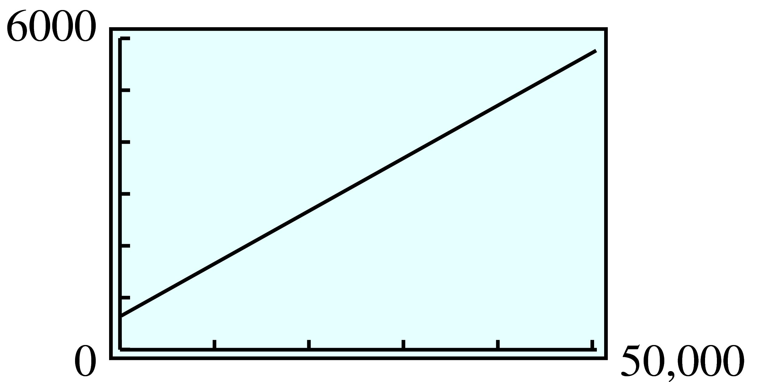
| \(t\) | \(0\) | \(5\) | \(10\) | \(15\) | \(20\) | \(25\) | \(30\) |
| \(N(t)\) | \(6000\) | \(7328\) | \(8951\) | \(10,933\) | \(13,353\) | \(16,310\) | \(19,921\) |