To write an algorithm that can learn, we need a way to track how well it is doing. Our absolute goal in training a neural network is to find a specific combination of weights and biases which minimize a cost function.
A cost function (sometimes called a ) is a mathematical yardstick that measures a neural network’s performance by calculating how far off its predictions are from the correct answers, outputting a single error score that we try to get as close to zero as possible. An example is the quadratic cost function or mean squared error.
If the actual outputs are approximately the same as the desired outputs for all training inputs, then the cost will be small. Conversely, if it is not, the cost will be large. The goal of our training algorithm is to find a set of weights and biases which make the cost as small as possible.
Imagine learning to shoot a basketball in total darkness. You can’t see the hoop, but someone calls out how many inches to the left or right your shot missed. Every shot gives you a specific error distance (your cost). Based on that feedback, you slightly tweak your arm angle and force (your weights and biases) for the next try. Over many throws, each small adjustment brings your shots closer and closer to a swish.
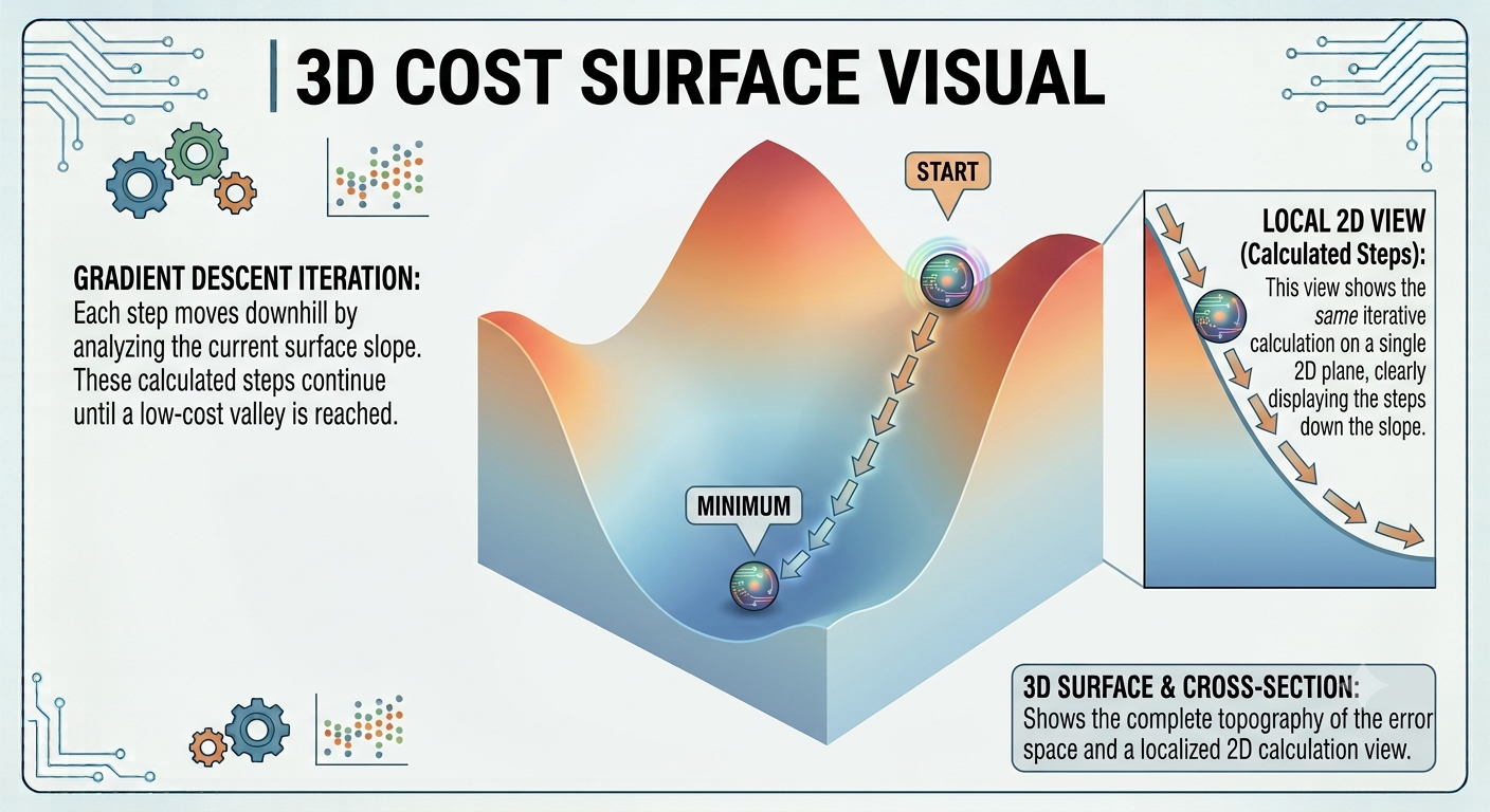
The Valley Analogy: The way the gradient descent algorithm works is to repeatedly compute the gradient and move in the opposite direction, “falling down” the slope of the valley.
Central 3D Surface Plot: Displays a continuous cost surface (error space). A ball labeled "START" begins near a high-cost peak and follows a sequence of downward arrows down the slope, coming to rest at the lowest valley labeled "MINIMUM."
Left Panel (Gradient Descent Iteration): Explains that each step moves downhill by analyzing the current surface slope, repeating until a low-cost valley is reached.
Right Panel (Local 2D View): Shows an inset 2D cross-section of the curve, illustrating the ball taking discrete, calculated steps down the slope toward the bottom.
Lower-Right Summary: Notes that combining the 3D surface and 2D cross-section shows both the overall error space topography and a localized view of the calculations.
We can visualize it as a ball rolling down into a valley. Notice that with our mathematical rule, gradient descent doesn’t reproduce real physical motion. In real life, a ball has momentum, and that momentum may allow it to roll across the slope, or even momentarily roll uphill. It’s only after the effects of friction set in that the ball is guaranteed to roll down into the valley.
To compute the exact direction down the valley, we technically need to average our calculations over all training inputs simultaneously. If the training set is very large, this can take a long time, and learning occurs slowly.
To speed up learning, we use stochastic gradient descent. This works by randomly choosing a small sample of training inputs, known as a mini-batch. By averaging the gradient over this small sample, we can quickly estimate the true direction we need to go, allowing us to make rapid, frequent updates to the weights and biases.
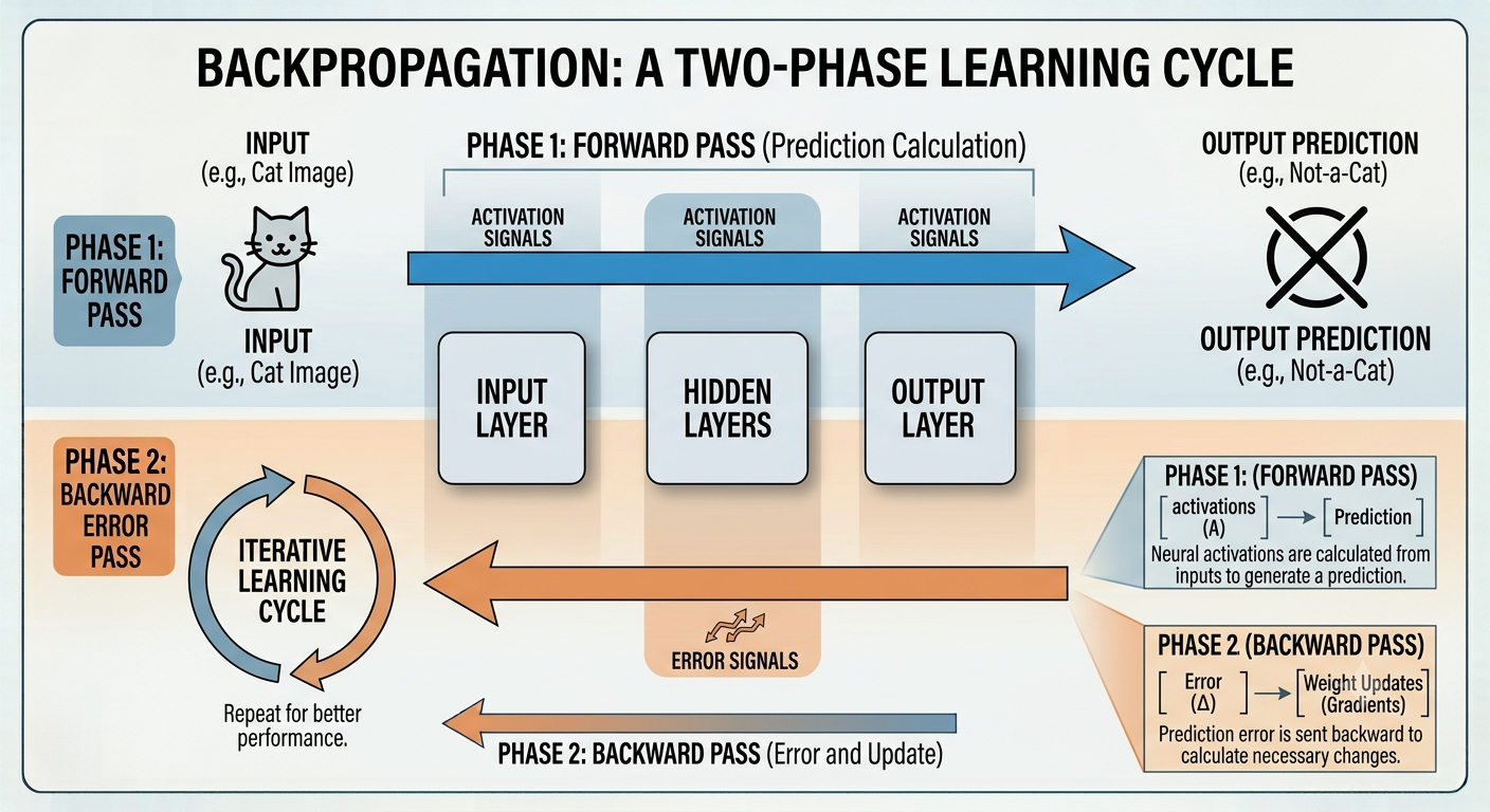
The backpropagation algorithm gives us a way of computing how quickly the cost changes when we make small changes to any weight or bias in the network. It allows us to calculate all of these partial derivatives simultaneously and extremely quickly.
Phase 1 (Forward Pass): An upper blue arrow points left-to-right from an input (e.g., a cat image) through the layers to generate an output prediction. Neural activations are calculated forward to form this guess.
Phase 2 (Backward Pass): A lower orange arrow points right-to-left from the output back through the hidden layers toward the input. Prediction error signals travel backward to compute required weight updates (gradients).
Figure6.4.2.The two-phase iterative cycle of backpropagation: a forward pass calculates network predictions, followed by a backward pass that transmits error signals to update weights.
These backpropagated errors provide the exact information needed to make a small step down the cost landscape using gradient descent. Through millions of these tiny, layer-by-layer adjustments, the network gradually learns, refining its internal parameters until it can reliably solve complex real-world problems.
Consider the difference between standard gradient descent and stochastic gradient descent (SGD). Which of the following statements are true? Select all that apply.
Standard gradient descent computes the gradient using the entire training dataset for each update, while SGD computes it using a small mini-batch.
Correct. The "stochastic" part refers to using random mini-batches rather than the full dataset to estimate the gradient.
SGD is typically faster per update than standard gradient descent because it processes fewer examples.
Correct. Think about the math—if you compute a gradient using 100 examples versus 100,000 examples, which calculation finishes faster? SGD’s speed advantage comes directly from processing less data per update.
Standard gradient descent will always find the global minimum of the cost function regardless of the network’s architecture.
Incorrect. This statement overpromises what gradient descent can achieve. Neural networks have non-convex cost functions with many local minima. While gradient descent will reduce the cost, it does not guarantee finding the global minimum.
SGD introduces randomness into the training process because each mini-batch provides a different estimate of the true gradient.
Correct. The randomness from mini-batch sampling is what makes SGD "stochastic." This noise can actually be beneficial, as it helps the network escape shallow local minima.
Using SGD rather than standard gradient descent guarantees the network will converge to a lower cost value.
Incorrect. This is an overstatement. SGD is not guaranteed to find a lower cost value than standard gradient descent. The noisy estimates mean SGD often converges to a slightly higher training cost, but it does so much faster and can sometimes find more generalizable solutions.