Section 3.2 Introduction to State Spaces
In AI, before an algorithm can search for a solution, we must first mathematically represent the problem itself. This representation is called the state space. Think of it as a vast map containing every possible configuration or “state” the problem can be in, from the starting moment to the final, solved state.
Rather than providing a computer with step-by-step instructions on how to solve a problem, we describe the problem in terms of states and allowable moves, enabling the AI agent to navigate the space and find a solution independently. An Agent (or Agentic AI) is AI that can autonomously take multiple actions to complete complex tasks. Example: AI that can research, write, and edit a report without step-by-step guidance.
Imagine you’re trying to find your way out of a maze. At any moment, you’re standing in one particular location—that’s your current state. The maze itself, with all its twists, turns, and dead ends, represents the state space: every possible location you could be in while trying to find the exit.
Subsection 3.2.1 Nodes, Arcs, and Relationships
The state space is typically visualized as a graph or a tree, a structure composed of two key elements:
-
Node: In the state space, each point, or position, is a node. A node represents a specific, instantaneous configuration or snapshot of the problem. The entire search process starts at the initial state (the root node) and aims to reach a goal state (a node that represents the solution).A state can be simple or composed of multiple variables. For example, in a warehouse delivery robot problem, a single state node might capture:
-
The robot’s current location (aisle 3, section B)
-
Whether it’s carrying a package
-
The time of day
The important thing to note is that a state only includes relevant information for solving the problem. The robot doesn’t need to remember what color its wheels are or the brand name on its side. -
-
Arcs and the relationship between nodes: The connections between nodes are called arcs (or edges). An arc represents an action, a move, or operation that transitions the problem from one state to another. These actions are defined by the rules of the problem. For example, in a travel map, an arc is a road connecting two cities.In the process of searching, when an algorithm moves from one node to the next, we define a relationship:
-
The node the search is moving from is the parent node.
-
The node the search is moving to is the child node or successor state.
A child node is generated by applying an action to its parent node. The goal of the entire search is to find a sequence of arcs (actions) that connect the initial state to the goal state—a complete, effective path. -
Subsection 3.2.2 Tic-Tac-Toe Example
Using tic-tac-toe as an example, we can visualize game states using a tree structure where each node represents a specific board configuration. Looking at Figure 3.2.1 below, let’s say you are player X while AI is player O; we see the initial state, the beginning of the game before any moves have been made. The empty board is the root node. From there, the AI has 9 possible actions for its first move because there are 9 available boxes in a tic-tac-toe grid. Each action leads to a new state, represented by the 9 branches in Figure 3.2.1. This movement from one state to another through an action is called a transition. Each time a player makes a move, the game transitions from the current state to a new state.
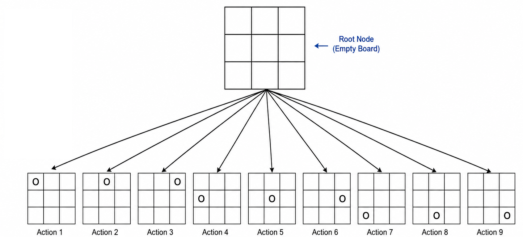
A tree diagram illustrating the state space for the first move in a tic-tac-toe game, where player O moves first. The diagram is structured vertically from top to bottom with evenly spaced, balanced branches. At the top is the root node, which displays an empty 3x3 tic-tac-toe grid representing the initial state before any moves have been made. From this root node, nine branches extend downward in a balanced tree formation, each leading to a node that displays a 3x3 tic-tac-toe grid showing the resulting board state. Each branch corresponds to one of the nine possible first moves for player O, labeled according to the position on the grid: Action 1 (top-left), Action 2 (top-center), Action 3 (top-right), Action 4 (middle-left), Action 5 (center), Action 6 (middle-right), Action 7 (bottom-left), Action 8 (bottom-center), and Action 9 (bottom-right). In each resulting node, the corresponding position on the 3x3 grid contains an O marking, indicating player O’s first move. The tree shows that from the empty board, there are exactly nine possible legal moves for the first player, each leading to a distinct board configuration.
After the first move is made, there are only 8 possible moves, no matter what the first move was. Figure 3.2.2 zooms in on just one branch from Figure 3.2.1—specifically, the branch where the AI placed its O in the center square (Action 5). Figure 3.2.2 shows your 8 possible moves after the AI’s first move. You can place an X in any of the 8 available boxes. Each of these moves represents another transition, moving the game from the center-O state to one of 8 new states.
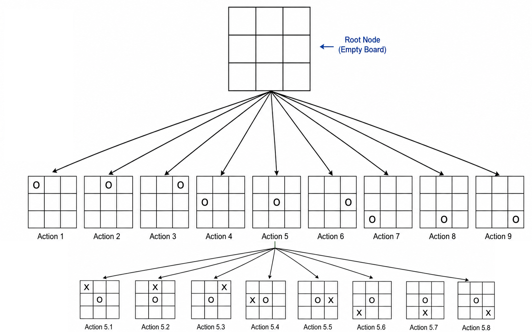
A tree diagram illustrating two levels of moves in a tic-tac-toe game, where player O moves first followed by player X. The diagram is structured vertically from top to bottom with a hierarchical branching pattern. At the top is the root node, which displays an empty 3x3 tic-tac-toe grid representing the initial state before any moves have been made.
From the root node, nine branches extend downward, each representing a possible first move for player O. These branches are labeled Action 1 through Action 9, corresponding to the nine positions on the tic-tac-toe grid. Each of these nine branches leads to a node displaying the resulting board state with an O placed in the corresponding position.
The Action 5 branch (representing O placed in the center square) is expanded further. From this node, which shows a 3x3 grid with O in the center, eight branches extend downward, labeled Action 5.1 through Action 5.8. Each branch represents a possible second move for player X, corresponding to the eight remaining empty positions on the grid. Each of these eight branches leads to a node displaying the resulting board state, showing a 3x3 grid with O in the center and X placed in one of the eight available positions: top-left, top-center, top-right, middle-left, middle-right, bottom-left, bottom-center, or bottom-right.
The other eight branches from the root (Actions 1, 2, 3, 4, 6, 7, 8, and 9) are shown as complete first-level paths with their corresponding O placed in the respective positions, but these branches are not expanded further, emphasizing that this diagram focuses specifically on the branch where O plays in the center position. The tree is evenly spaced at the first level, with the Action 5 branch receiving additional depth while the others remain unexpanded.
AI uses these state spaces to work towards a goal state. Let’s fast forward to a state where only 3 moves are left. Figure 3.2.3 shows a state with only 3 empty squares remaining. The goal state is any state where the AI wins the game, so the AI will evaluate its possible actions to see which ones bring it closer to that goal state. Each action the AI considers is a potential transition, moving the game from the current state toward a winning state. By exploring these state spaces and the transitions between them, the AI can look ahead and choose actions that lead toward victory.
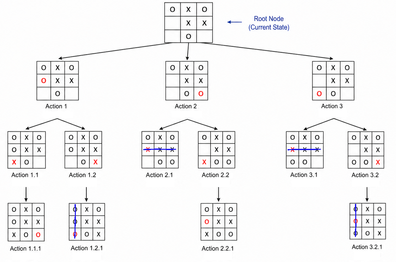
A tree diagram illustrating three levels of moves in a tic-tac-toe game. The diagram is structured vertically from top to bottom with a hierarchical branching pattern. At the top is the root node, which displays a 3x3 tic-tac-toe grid representing the current state of the game with three empty squares remaining.
From the root node, three branches extend downward, labeled Action 1, Action 2, and Action 3. Each branch represents a possible move for player O, corresponding to one of the three remaining empty positions on the grid. Each node at this level displays the resulting board state with O placed in the corresponding position.
At the second level, each action branches further. Action 1 leads to two branches labeled Action 1.1 and Action 1.2. Action 2 leads to two branches labeled Action 2.1 and Action 2.2. Action 3 leads to two branches labeled Action 3.1 and Action 3.2. Each of these branches represents a possible response move for player X from the resulting state after O’s first action. Each node at this level displays the resulting board state with X placed in the corresponding position.
At the third level, Action 1.1 leads to Action 1.1.1, Action 1.2 leads to Action 1.2.1, Action 2.2 leads to Action 2.2.1, and Action 3.2 leads to Action 3.2.1, representing possible moves for player O from the resulting states. Action 2.1 and Action 3.1 are shown without further branching. Each node at this level displays the resulting board state with O placed in the corresponding position.
Subsection 3.2.3 The Problem-Solving Process
With states and actions defined, an AI agent solves a problem by navigating its state space through a structured four-part framework:
-
Initial State: The AI determines its starting point within the state space.
-
Goal State: The AI identifies the target configuration or conditions that define a successful solution.
-
Actions: The AI evaluates the valid transitions available from its current node to adjacent nodes.
-
Search: The AI systematically explores sequences of actions to discover a valid sequence of transitions connecting the initial state to the goal state.
During the search process, the AI traverses the state space by evaluating candidate actions and transitioning through successor states. As it evaluates different branches of the state space tree, the algorithm may encounter dead-end nodes that offer no further valid moves, or loops that return to previously visited states. The objective of the search algorithm is to navigate past these inefficient paths and isolate an optimal sequence of actions that leads directly to the goal state.
Subsection 3.2.4 Real-World State Spaces
State spaces are used throughout AI. Here are some common examples:
-
Route Planning
-
States: Cities, intersections, or specific locations
-
Actions: Driving along roads between locations
-
Goal: Reaching your destination
-
-
Puzzle Solving
-
States: Arrangements of puzzle pieces
-
Actions: Moving pieces according to the rules
-
Goal: A specific arrangement (the solution)
-
-
Task Scheduling
-
States: Which tasks are completed and which remain
-
Actions: Starting or completing a task
-
Goal: All tasks completed
-
-
Game Playing
-
States: Positions of pieces on a board
-
Actions: Making a legal move
-
Goal: Achieving a winning position
-
Subsection 3.2.5 Important Characteristics of State Spaces
State spaces can be enormous. The game of chess has approximately \(10^{47}\) possible states (that’s a 1 with 47 zeros after it). Yet AI systems can play chess brilliantly by exploring only a tiny fraction of these states intelligently.
Some state spaces are small enough to explore completely. Others are so vast that we must use clever strategies to find solutions without examining every possibility.
Subsection 3.2.6 The Challenge of Representation
How you represent states matters tremendously. A well-designed state representation captures everything relevant and nothing irrelevant. It makes the problem easier to solve.
Consider planning a delivery route through a city:
-
Too simple: Just the city name (not enough detail for route planning)
-
Too complex: The exact address, traffic conditions, weather, time of day, and the driver’s mood (too much detail)
-
Just right: Location coordinates and which streets connect to which
Finding the right balance is part of the art of AI problem-solving.
You have attempted of activities on this page.

