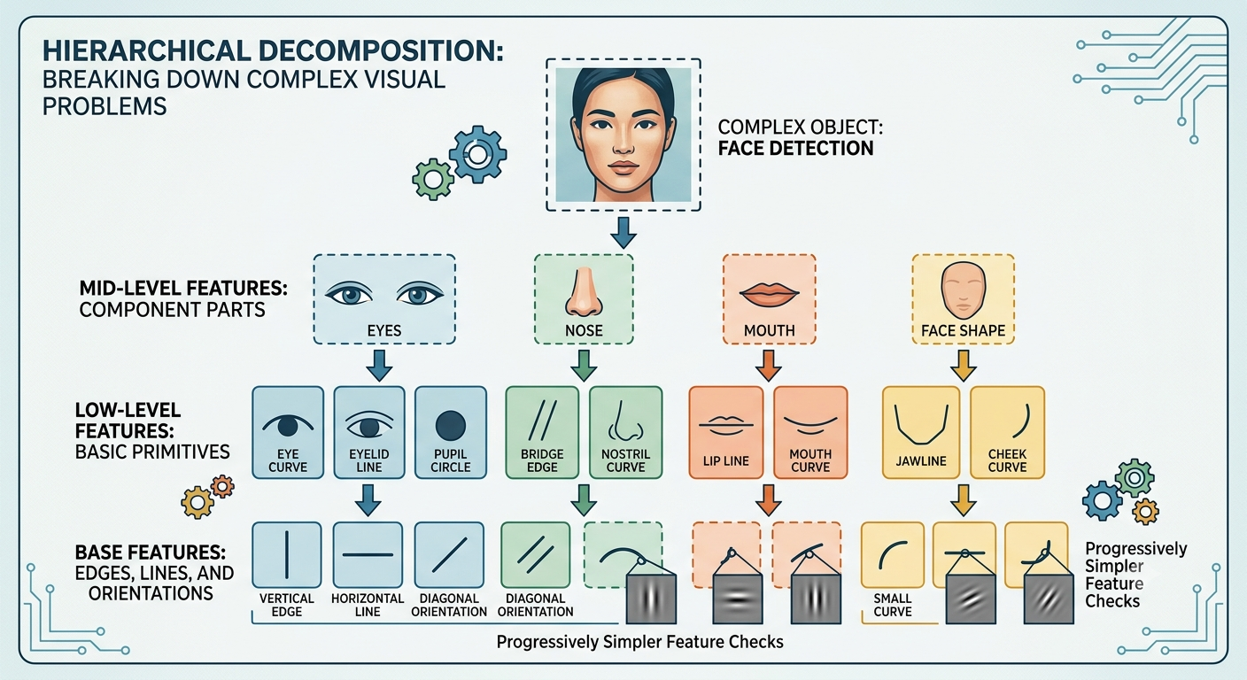
To build intuition about how networks function, let’s look at how we might approach a complex problem like face detection. We could attack this by using the pixels in an image as input to a neural network.
If the answers to several of these questions are “yes”, or even just “probably yes”, then we’d conclude that the image is likely to be a face. Conversely, if the answers to most of the questions are “no”, then the image probably isn’t a face.
It’s also plausible that the sub-problems can be further decomposed. Suppose we’re considering the question: “Is there an eye in the top left?” This can be decomposed into questions such as: “Is there an eyebrow?”; “Are there eyelashes?”; “Is there an iris?”; and so on.
A structured tree diagram titled "HIERARCHICAL DECOMPOSITION: BREAKING DOWN COMPLEX VISUAL PROBLEMS" illustrates the multi-level feature breakdown used in computer vision tasks like face detection.
An arrow points down to the second tier, labeled "MID-LEVEL FEATURES: COMPONENT PARTS." This level breaks the face down into four distinct, color-coded component categories: "EYES" (blue), "NOSE" (green), "MOUTH" (orange), and "FACE SHAPE" (yellow).
Finally, arrows lead down to the bottom tier, labeled "BASE FEATURES: EDGES, LINES, AND ORIENTATIONS." At this foundational level, primitives are reduced to raw geometric elements and directional filters, such as "VERTICAL EDGE," "HORIZONTAL LINE," "DIAGONAL ORIENTATION," "SMALL CURVE," and pixel-level Gabor/edge filter patches.
The end result is a network which breaks down a very complicated question—does this image show a face or not—into very simple questions answerable at the level of single pixels.
Think of hierarchical learning like building with toy blocks. Instead of manufacturing a whole toy castle out of plastic all at once, you assemble simple individual blocks into walls, combine walls into towers, and connect towers into a finished castle. Deep layers work the exact same way: early layers assemble raw pixels into simple edges, middle layers combine edges into shapes like eyes or noses, and final layers combine those shapes to identify an entire face.
So far, we have studied what are called fully connected neural networks, in which all of the units at one layer are connected to all of the units in the next layer. This is a good arrangement when we don’t know anything about what kind of mapping from inputs to outputs we will be asking the network to learn to approximate.
But if we do know something about our problem, it is better to build it into the structure of our neural network. Doing so can save computation time and significantly diminish the amount of training data required to arrive at a solution that generalizes robustly.
The reason deep nets perform far better on many problems than shallow neural networks (networks with just a single hidden layer) is their ability to build up a complex hierarchy of concepts. It’s a bit like the way conventional programming languages use modular design and ideas about abstraction to enable the creation of complex computer programs.
Comparing a deep network to a shallow network is a bit like comparing a programming language with the ability to make function calls to a stripped-down language with no ability to make such calls. Abstraction takes a different form in neural networks than it does in conventional programming, but it’s just as important.
As neural networks evolved, specific arrangements of layers were developed to process different types of data structures. One very important application domain of neural networks, where the methods have achieved an enormous amount of success in recent years, is signal processing. Signals might be spatial (in two-dimensional camera images or three-dimensional depth or CAT scans) or temporal (speech or music). If we know that we are addressing a signal-processing problem, we can take advantage of invariant properties of that problem.
Convolutional Neural Networks (CNNs): In fully connected layers, the inputs are treated as a simple, flat vertical line of neurons. In a convolutional net, it helps to think instead of the inputs as a square or two-dimensional array of pixels, whose values correspond to pixel intensities (such as three integer values encoding intensity levels in red, green, and blue color channels).
The set of pixels we will have to take into consideration to find an object will be near one another in the image. We won’t have to consider some combination of pixels in the four corners of the image in order to see if they encode an object.
The pattern of pixels that characterizes an object is the same no matter where in the image the object occurs. Objects don’t look different if they’re on the left or the right side of the image.
To exploit these properties, convolutional networks pass a filter (also called a convolutional kernel) along the image, multiplying the filter’s values by the corresponding pixel values in each local neighborhood and summing them up at each step. This process of applying the filter to the image to create a new image is called convolution.
Filter Size: The dimensions of the local window scanning the input pixels (such as a 5-by-5 square). This area of an input image that a filter is being applied to is called the receptive field.
Padding: How many extra pixels—typically with value 0—we add around the edges of the input. We generally pad the input image with 0 values to ensure that the output image maintains a proper shape when accessing pixels beyond the bounds of the original image.
Stride: The spacing at which we apply the filter to the image. A stride of one moves the window step-by-step. If we "skip" and apply the filter only at wider intervals, the stride increases, producing a resulting image of a smaller size.
Channels: Applying multiple filters to the original image results in new images called channels. Stacking all these new images up creates a cube of data, and these multi-dimensional chunks of data are called tensors.
Max Pooling Layers: It is typical to structure filter banks into a pyramid, in which the image sizes get smaller in successive layers of processing. The idea is that we find local patterns, like bits of edges in the early layers, and then look for patterns in those patterns. Having a stride greater than one makes the images smaller, but does not necessarily aggregate information over that spatial range.
Another common layer type, which accomplishes this aggregation, is max pooling. A max pooling layer operates like a filter, but has no weights. It is a pure functional layer that simply returns the maximum value in its field. As a result of applying a max pooling layer, we don’t keep track of the precise location of a pattern. This helps our filters to learn to recognize patterns independent of their location.
Recurrent Neural Networks (RNNs): While CNNs focus on spatial, grid-like data, other networks are explicitly built for temporal or sequential problems. In standard networks, there are no loops—information is always fed forward, never fed back.
In these models, neurons turn on for a brief moment and then go quiet. Before they shut off, they trigger neighboring neurons to fire shortly after, creating a chain reaction over time. This continuous looping effect is what allows the network to remember past information. Think of these neurons like a row of falling dominoes that loop back on themselves. One neuron fires briefly, triggers the next one a moment later, and shuts off, creating a continuous wave of activity that keeps the memory of past inputs alive in the network.
After each filter layer there is generally a ReLU layer; there may be multiple filter/ReLU layers, then a max pooling layer, then some more filter/ReLU layers, then max pooling. Once the output is down to a relatively small size, there is typically a last fully-connected layer, leading into an activation function that produces the final classification output.
The critical point for us is that this is all just a big neural network, which takes an input and computes an output. The mapping is a differentiable function of the weights, which means we can adjust the weights to decrease the loss by performing gradient descent, and we can compute the relevant gradients using back-propagation. This will be discussed more in the next section.