Section 6.2 Inputs, Weights, and Biases

Inputs, weights, and biases are three of the most fundamental concepts in artificial neural networks (ANNs), and the relationship between them forms the backbone of the entire system.

Look Closer...

Think of an artificial neuron like making a group decision with friends about where to eat dinner. Each friendโ€™s suggestion is an "input." The friends you trust most on food recommendations get higher "weight" in your decision. Your baseline moodโ€”whether you are starving and eager to agree to anything, or picky and hard to satisfyโ€”acts as your "bias." Combining how much you weight everyoneโ€™s input with your internal baseline determines whether you decide to say yes or no.
Subsection 6.2.1 The Role of Each Component

To understand how a neuron computes an answer, we first break down the three primary building blocks that drive its calculation:
Inputs
Inputs represent the evidence or raw features passed forward from the preceding layer of neurons. In the very first layer of a network (the input layer), these values correspond to the raw data itself, such as the pixel intensities of an image. In subsequent layers, the inputs are the activation outputs generated by the hidden neurons that came before them.
Weights
Weights are parameters that express the importance of the respective inputs to the output. You can think of the network as weighing up evidence. If a particular input is highly significant to the correct decision, it is assigned a large weight. Conversely, if an input is of little consequence, its weight will hover close to zero. Negative weights represent evidence that actively contradicts or suppresses a particular outcome.
Biases
The bias is a measure of how easy it is to get the neuron to output a 1. To put it in more biological terms, the bias is a measure of how easy it is to get the artificial neuron to fire. For a neuron with a really big bias, itโ€™s extremely easy to output a 1. But if the bias is very negative, then itโ€™s difficult for the neuron to fire. The bias serves as an internal threshold, determining how much total weighted evidence a neuron must accumulate before it shifts its state.

Subsection 6.2.2 How the Layer Activates

What do we mean by โ€œactivatesโ€? To understand this phrase, recall our biological analogy. In the human brain, a neuron fires (or activates) when it receives a strong enough electrical signal. In an ANN, a layer activates when it takes incoming data, weighs the evidence, and calculates a final numeric output. โ€œHow a layer activatesโ€ is simply the mechanical process of deciding how strongly each neuron will fire its signal forward.
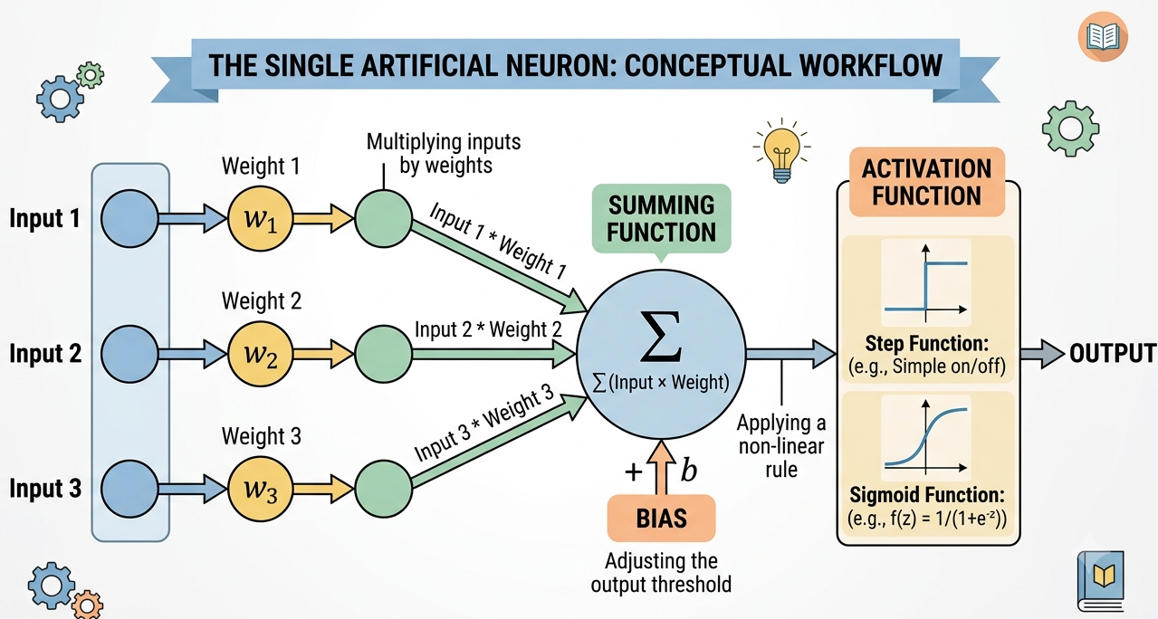
Diagram showing inputs multiplied by weights, summed together with bias, and passed to an activation function.
A flow diagram illustrates the step-by-step mathematical process inside a single artificial neuron. It starts with three distinct input values, labeled Input 1, Input 2, and Input 3. Each input is multiplied by its corresponding weight parameter, denoted as w1, w2, and w3. Text above these connections explains this action as "Multiplying inputs by weights."
The resulting products (e.g., Input 1 * Weight 1) are channeled into a central, blue circular node representing the summing function, indicated by a large summation symbol (ฮฃ). The text "ฮฃ(Input ร— Weight)" details this operation. A separate orange block for "BIAS" adds a parameter โ€™bโ€™ directly into the summation node, with text explaining that the bias acts as "Adjusting the output threshold."
An arrow carries the combined sum to an orange rectangle labeled "ACTIVATION FUNCTION." This step is described as "Applying a non-linear rule." The box includes graphical representations of common activation functions: a "Step Function" with a chart showing a sharp on/off threshold, and a "Sigmoid Function" with an S-curve chart and its corresponding formula, f(z) = 1/(1+eโปแถป). A final output value, labeled "OUTPUT," emerges from the activation function node, completing the workflow.
Figure 6.2.1. The single artificial neuron: conceptual workflow.
To calculate the active signal of a single neuron in a new layer, the network performs a straightforward, step-by-step process:
  1. Weighing the Evidence: We multiply each incoming activation from the previous layer of neurons by its corresponding weight.
  2. Summing the Values: We add all of these weighted inputs together to create a single sum.
  3. Adding the Bias: We add the neuronโ€™s individual bias to this sum.
  4. Applying the Activation Function: Finally, we pass this entire total through our activation function (the sigmoid function) to get the neuronโ€™s final output.
Applying this process to all the neurons at once gives us a global way of thinking about how layers interact: we apply the weight matrix to the previous layerโ€™s activations, add the bias vector, and apply our activation function to the total.

Subsection 6.2.3 Activation Functions

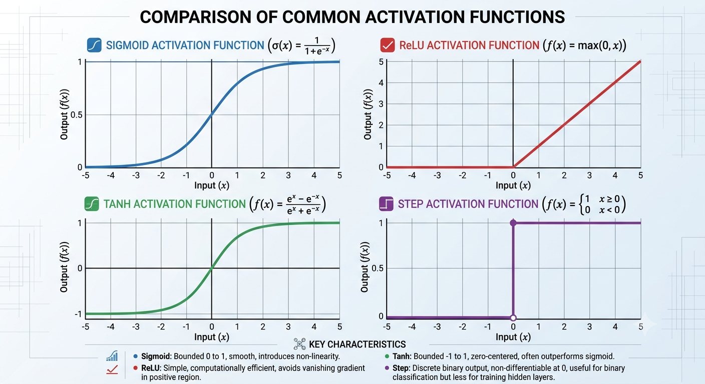
The activation function acts as a mathematical filter that shapes the final output of the neuron, compressing the calculated value into a predictable range (such as a smooth gradient between 0 and 1). While we have focused on the sigmoid function as our primary example, modern AI utilizes a variety of other activation functions to filter signals differently depending on the specific problem the network is trying to solve. Two of the most common include:
Rectified Linear Unit (ReLU)
A simple, fast activation function that outputs the input directly if it is positive, and outputs zero if it is negative (mathematically, \(f(x) = \max(0, x)\)). It is the default choice for many deep neural networks because it helps prevent training bottlenecks.
Hyperbolic Tangent (tanh)
An S-shaped curve similar to the sigmoid function, but it maps input values to a range between -1 and 1. Because its outputs are zero-centered, it often makes optimization easier during training.
A grid of four graphs, each showing the curve and formula for a different neural network activation function: Sigmoid, ReLU, Tanh, and Step.
A 2x2 grid of graphs compares four common activation functions. Each graph includes a curve of the function, its name, and its mathematical formula.
The top-left graph shows the "SIGMOID ACTIVATION FUNCTION (ฯƒ(x) = 1 / (1 + eโปหฃ))". A blue S-shaped curve rises from near 0 at input -5 to near 1 at input 5. It passes through the y-intercept at f(0) = 0.5.
The top-right graph shows the "ReLU ACTIVATION FUNCTION (f(x) = max(0, x))". A red line is flat at y=0 for all negative inputs (from -5 to 0) and then rises diagonally (where y=x) for all positive inputs (from 0 up to 5).
The bottom-left graph shows the "TANH ACTIVATION FUNCTION (f(x) = (eหฃ - eโปหฃ) / (eหฃ + eโปหฃ))". A green S-shaped curve, similar to the sigmoid, is zero-centered. It rises from near -1 at input -5, passes through the origin (0, 0), and reaches near 1 at input 5.
The bottom-right graph shows the "STEP ACTIVATION FUNCTION (f(x) = 1 if x โ‰ฅ 0; 0 if x < 0)". A purple plot shows a function that is flat at y=0 for all negative inputs, jumps directly to 1 at input 0 (represented by a solid dot at (0,1) and an open dot at (0,0)), and remains flat at y=1 for all positive inputs.
A "KEY CHARACTERISTICS" section at the bottom provides short descriptions of each function, such as "Sigmoid: Bounded 0 to 1," "ReLU: computationally efficient," "Tanh: zero-centered," and "Step: Discrete binary output."
Figure 6.2.2. Graphs comparing common activation functions: Sigmoid, Step, ReLU, and tanh.
Without an activation function, a neural network would merely perform basic addition and multiplication. This means the entire system would collapse into a simple, flat linear calculation, making it mathematically impossible for the network to understand or infer complex, non-linear patterns. The non-linear nature of the activation function bends the signal, enabling the network to learn intricate and highly abstract behaviors.

Reading Questions 6.2.4 Reading Questions

1.

You have attempted of activities on this page.