Project 2.5.1. Project—Modeling a Pandemic.
On December 31, 2019, the city of Wuhan in China reported an outbreak of a novel coronavirus (COVID-19). It is the seventh member of the coronavirus family, together with MERS-CoV and SARS-CoV, that can spread to humans. The virus is spreading rapidly. As of January 10, 2021, over 89 million people worldwide have been infected, including over 1.9 million deaths. The World Health Organization (WHO) has declared the outbreak as a pandemic.
1
Johns Hopkins Coronavirus Resource Center, 2021.
coronavirus.jhu.edu. Accessed 10 January 2021.
2
This project is adapted from Jue Wang (2020), “6-016-S-PandemicModeling,”
www.simiode.org/resources/7518
The word “pandemic” comes from the Greek word “pandemos,” meaning “pertaining to all people.” Pandemics are usually caused by an infectious agent that is capable of rapidly spreading. An epidemic is specific to one city, region, or country, but a pandemic spreads beyond national borders, possibly worldwide. The 1918 Spanish flu was the worst pandemic in modern human history. It infected 500 million people around the world and resulted in the deaths of over 50 million people. Increased travel and mobility have increased the likelihood of new diseases spreading. Table 2.5.1 lists the major epidemics and pandemics that have occurred over time. The recent ones are SARS, swine flu, Ebola, MERS, and COVID-19.
3
Centers for Disease Control and Prevention. 2019. 1918 influenza pandemic (H1N1 virus).
www.cdc.gov/flu/pandemic-resources/1918-pandemic-h1n1.html. Accessed 10 January 2021.
4
World Economic Forum. 2021. A visual history of pandemics.
www.weforum.org/agenda/2020/03/a-visual-history-of-pandemics. Accessed 10 January 2021.
| Name | Time Period | Type/Pre-Human Host | Death Toll |
| Antonine Plague | 165–180 | Believed to be smallpox or measles | 5 million |
| Plague of Justinian | 541–542 | Yersinia pestis bacteria/rats, fleas | 30–50 million |
| Japanese Smallpox Epidemic | 735–737 | Variola major virus | 1 million |
| Black Death | 1347–1351 | Yersinia pestis bacteria/rats, fleas | 200 million |
| New World Smallpox Outbreak | 1520 onwards | Variola major virus | 56 million |
| Great Plague of London | 1665 | Yersinia pestis bacteria/rats, fleas | 100,000 |
| Italian Plague | 1629–1631 | Yersinia pestis bacteria/rats, fleas | 1 million |
| Cholera Pandemics 1–6 | 1817–1923 | V. cholerae bacteria | 1+ million |
| Third Plague | 1885 | Yersinia pestis bacteria/rats, fleas | 12 million (China and India) |
| Yellow Fever | Late 1800s | Virus/Mosquitos | 100,000–150,000 (U.S.) |
| Russian Flu | 1889–1890 | Believed to be H2N2 (avian origin) | 1 million |
| Spanish Flu | 1918–1919 | H1N1 virus/Pigs | 40–50 million |
| Asian Flu | 1957–1958 | H2N2 virus | 1.1 million |
| Hong Kong Flu | 1968–1970 | H3N2 virus | 1 million |
| HIV/AIDS | 1981–present | Virus/Chimpanzees | 25–35 million |
| SARS | 2002–2003 | Coronavirus/Bats, civets | 770 |
| Swine Flu | 2009–2010 | H1N1 virus/Pigs | 200,000 |
| Ebola | 2014–2016 | Ebola virus/Wild Animals | 11,000 |
| MERS | 2015–present | Coronavirus/Bats, camels | 850 |
| COVID-19 | 2019–present | Coronavirus/Unknown (possibly bats) | 7.1 million (as of Jan 19, 2026) |
Infectious disease modeling is an essential part of the effort to minimize the spread. A well-designed model not only can help predict the likely course of an epidemic, but also can reveal the most promising and realistic strategies for containing it.
Following the SIR model in Subsection 2.1.3, we will assume that we have a closed population of size \(N\text{,}\) where immigration, emigration, and birth do not play an important role. We will also ignore any deaths that are not related to our disease.
We will assume that each individual in the population falls into one of the following categories:
\begin{align*}
s(t) \amp = \text{Susceptible individuals}\\
i(t) \amp = \text{Infected individuals}\\
r(t) \amp = \text{Removed individuals}
\end{align*}
Susceptible individuals are those who do not yet have the disease and can catch the disease from infected individuals. Individuals enter the removed population by either recovering from the disease or dying. If an infected individual recovers, then the individual is immune to the disease. Schematically, we can represent the effect of the disease by the diagram
\begin{equation*}
s \longrightarrow i \longrightarrow r.
\end{equation*}
Since the population is closed, we know that
\begin{equation*}
s(t) + i(t) + r(t) = N.
\end{equation*}
It may seem more natural to work with population counts, but some of our calculations will be simpler if we use the fractions instead. Therefore, we normalize the dependent variables by the total population to represent the fraction of the total population in each group. The two sets of dependent variables are proportional to each other, so either set will give us the same information about the progress of the epidemic
\begin{align*}
S(t) \amp = s(t)/N = \text{the fraction of susceptible individuals}\\
I(t) \amp = i(t)/N = \text{the fraction of infected individuals}\\
R(t) \amp = r(t)/N = \text{the fraction of removed individuals}\\
1 \amp = S(t) + I(t) + R(t)\text{.}
\end{align*}
The SIR model is described by the nonlinear system of below, where \(\alpha\) is the transmission rate and \(\beta\) is the recovery rate.
\begin{align*}
\frac{dS}{dt} \amp = - \alpha SI\\
\frac{dI}{dt} \amp = \alpha SI - \beta I\\
\frac{dR}{dt} \amp = \beta I.
\end{align*}
To understand this model, let us analyze the differential equations and parameters. The transmission rate \(\alpha\) is the product of two factors: the rate of contact and probability of transmission. \(\alpha\) describes the fraction of those contacts that may result in infection, or it can be interpreted as the expected number of people an infected person infects per day. The function \(\lambda(I) = \alpha I\) is the rate at which susceptible individuals become infectious, called the force of infection. The rate of change of the susceptible population is negative the force of infection times the number of susceptible, leading to \(dS/dt = - \alpha SI\text{.}\)
The recovery rate \(\beta\) is the rate at which infected individuals get over the disease, that is the proportion of infected recovering per day, thus the rate of change of the recovered population is \(\beta I\text{,}\) leading to \(dR/dt = \beta I\text{.}\) Importantly, the parameter \(\beta\) is measured in \(1/\text{time}\) and \(1/\beta\) can be interpreted as the average time to recover, or the number of days an infected person has and can spread the disease.
The equation \(dI/dt = \alpha SI - \beta I\) now makes sense. The rate at which the fraction of infected individuals changes is the rate at which the fraction of susceptible minus the rate at which the fraction of individuals recover or
\begin{equation*}
\frac{dI}{dt} = \alpha SI - \beta I.
\end{equation*}
(a)
Using Sage, we can plot the solutions, and visualize the interaction of the three groups. Consider the initial population fractions \(S(0) = 0.99\text{,}\) \(I(0) = 0.01\text{,}\) \(R(0) = 0\text{,}\) \(\alpha = 1\text{,}\) \(\beta = 0.2\text{,}\) and a time period of 30 days. Adjust the parameters values to examine different behaviors and view the changes in action. What do you observe by increasing or decreasing \(\alpha\text{?}\)
(b) Basic Reproduction Number \(R_0\).
The basic reproduction number \(R_0\text{,}\) is introduced to measure the transmission potential of a disease. It is the expected number of secondary infections produced by a single infective. For example, if the \(R_0\) for measles in a population is 16, then we would expect each new case of measles to produce 16 new secondary cases over the period of time during which the infected individual can actually spread the disease. The reproduction number is affected by several factors: the rate of contacts in the host population, the probability of infection being transmitted during contact, and the duration of infectiousness. In the SIR model described above,
\begin{equation*}
R_0 = \frac{\alpha}{\beta}.
\end{equation*}
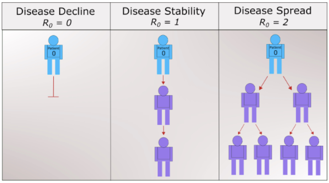
Simply put, \(R_0\) is a metric of how contagious a disease is. It can capture three basic scenarios (Figure 2.5.2). If \(R_0 \lt 1\text{,}\) on average, an infected person infects less than one person. The disease is expected to stop spreading. If \(R_0 = 1\text{,}\) an infected person infects an average of one person. The disease spread is stable, or endemic. If \(R_0 \gt 1\text{,}\) on average, an infected person infects more than one person. The disease is expected to increasingly spread in the absence of intervention. Measles is one of the most contagious with a range of 12–18 for the reproduciton number. Estimates of \(R_0\) for COVID-19 vary in the range of 2–2.5.
5
World Economic Forum. 2021. A visual history of pandemics.
www.weforum.org/agenda/2020/03/a-visual-history-of-pandemics Accessed 10 January 2021.
6
The Johns Hopkins University. 2021. Coronavirus: COVID-19 Terms You Should Know.
www.hopkinsmedicine.org/health/conditions-and-diseases/coronavirus/COVID-19-terms Accessed 10 January 2021.
(i)
Examine the system
\begin{align*}
\frac{dS}{dt} \amp = - \alpha SI\\
\frac{dI}{dt} \amp = \alpha SI - \beta I.
\end{align*}
According to the differential equation for \(dI/dt\text{,}\) under what conditions will \(I(t)\) be increasing? decreasing? What does this mean about the spread of the disease? Using this result, explain whether quarantine will be effective against the disease.
(ii)
Show that
\begin{equation*}
\frac{dI}{dS} = -1 + \frac{1}{R_0S}.
\end{equation*}
Two features of this new equation are particularly worth noting.
-
The only parameter that appears is \(R_0\text{,}\) the reproduction number.
-
The equation is independent of time. That is, what we learn about the relationship between \(S\) and \(I\) must be true for the entire duration of the pandemic.
Compute \(d^2I/dS^2\text{.}\) Determine when the number of infected will begin to decrease. Compare this to your result from Task 2.5.1.b.i.
Hint.
Use the chain rule.
(iii)
Show that \(I\) must have the form
\begin{equation*}
I = -S + \frac{1}{R_0} \ln S + C,
\end{equation*}
where \(C\) is a constant.
(iv)
For a disease such as COVID-19, \(I(0) \approx 0\) and \(S(0) \approx 1\text{.}\) A long time after the onset of the epidemic, we have \(\lim_{t \to \infty} I(t) = I_\infty\) approximately \(0\) again, and \(S_\infty = \lim_{t \to \infty} S(t)\) has settled to its steady state value, observable as the fraction of the population that did not get the disease. Explain why
\begin{equation*}
R_0 = \frac{\ln S_\infty}{S_\infty - 1}.
\end{equation*}
(v)
Describe the meaning and significance of “herd immunity.” How can vaccination lead to herd immunity?
(c) Your Final Report.
You have been commissioned to write a report on the COVID-19 pandemic to the state health department. In particular, your task is to explain what the meaning of \(R_0\) and its relationship to “herd immunity”. Your final report should contain a one-page executive summary. The executive summary should summarize your work in such a way that the reader can rapidly become acquainted with the material. It should contain a brief description of the problem, important background information, a discussion of pertinent assumptions, a short description of your methodology, concise analysis, and your main conclusions. Assume the reader is familiar with the basics of calculus and differential equations, so there is no need to walk through every step of your solution process or include equations. However, you should still describe the processes and mathematical techniques you used to reach your conclusions and explain why you used them. Refer the reader to the appendices as needed.
Appendices should be neatly formatted and present information in a logical manner. DO NOT simply print out Sage code. Consolidate your results and provide a short explanation of what it is the reader is seeing while also highlighting key pieces of information in the appendix.
-
Appendix A—Answers and analysis
-
Additional Appendices—Include additional appendices as necessary.
Other models include SEIR, SEIS, SEAIR, MSIR, MSEIR, and MSEIRS. For many infections, there is an incubation period during which individuals have been infected but are not yet infectious themselves. During this period the individual is in class E (for exposed), leading to the SEIR model. The SEIS model is like the SEIR except that no immunity is acquired at the end. In the E class, a significant number of persons may never develop symptoms, but they are capable of transmitting the disease, introducing an additional compartment A, and thus SEAIR. For many infections, such as measles, babies are not born into the susceptible compartment but are immune to the disease for the first few months of life due to protection from maternal antibodies. The M class contains infants with maternally derived immunity (or passive immunity). The MSEIRS model is similar to the MSEIR, but the immunity in the R class would be temporary, so that individuals would regain their susceptibility when the temporary immunity ended.
