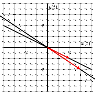
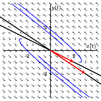
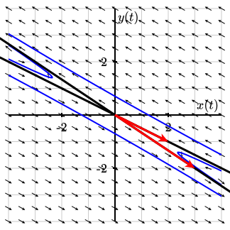
Section 3.3 Phase Plane Analysis of Linear Systems

In Section 3.2, we learned how to solve the system
\begin{equation*} \begin{pmatrix} dx/dt \\ dy/dt \end{pmatrix} = \begin{pmatrix} a & b \\ c & d \end{pmatrix} \begin{pmatrix} x \\ y \end{pmatrix} = A \begin{pmatrix} x \\ y \end{pmatrix} \end{equation*}
provided the system has distinct real eigenvalues. If \(A\) has distinct real eigenvalues \(\lambda\) and \(\mu\) with eigenvectors \(\mathbf u\) and \(\mathbf v\text{,}\) respectively, then the general solution of the system is
\begin{equation*} \mathbf x(t) = c_1 e^{\lambda t} \mathbf u + c_2 e^{\mu t} \mathbf v. \end{equation*}
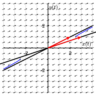
Furthermore, we can use the general solution of such a system to find the straight-line solutions to the system. If \(c_2 = 0\text{,}\) then all solutions will lie along the line in the \(xy\)-plane that contains the vector \(\mathbf u\text{.}\) Similarly, if \(c_1 = 0\text{,}\) then all solutions will lie along the line in the \(xy\)-plane that contains the vector \(\mathbf v\text{.}\)

Subsection 3.3.1 The Case \(\lambda_1 \lt 0 \lt \lambda_2\)

Example 3.3.1.

The system
\begin{align*} x' \amp = x + 3y\\ y' \amp = x - y \end{align*}
can be written in matrix form \(\mathbf x' = A \mathbf x\text{,}\) where
\begin{equation*} A = \begin{pmatrix} 1 & 3 \\ 1 & -1 \end{pmatrix}. \end{equation*}
The eigenvalues of \(A\) are \(\lambda = -2\) or \(\lambda = 2\) with eigenvectors \(\mathbf u = (1, -1)\) and \(\mathbf v = (3,1)\text{,}\) respectively. Therefore, the straight-line solutions must be lines containing \(\mathbf u\) and \(\mathbf v\) (Figure 3.3.2).
Diagram Exploration Keyboard Controls
Key Action
Enter, A Activate keyboard driven exploration
B Activate menu driven exploration
Escape Leave exploration mode
Cursor down Explore next lower level
Cursor up Explore next upper level
Cursor right Explore next element on level
Cursor left Explore previous element on level
X Toggle expert mode
W Extra details if available
Space Repeat speech
M Activate step magnification
Comma Activate direct magnification
N Deactivate magnification
Z Toggle subtitles
C Cycle contrast settings
T Monochrome colours
L Toggle language (if available)
K Kill current sound
Y Stop sound output
O Start and stop sonification
P Repeat sonification output
Figure 3.3.2. Straight-line solutions
Let us consider the special case of the system \({\mathbf x}' = A {\mathbf x}\text{,}\) where \(\lambda_1 \lt 0 \lt \lambda_2\) and
\begin{equation*} A = \begin{pmatrix} \lambda_1 & 0 \\ 0 & \lambda_2 \end{pmatrix}. \end{equation*}
Since this is a decoupled system,
\begin{align*} \frac{dx}{dt} & = \lambda_1 x\\ \frac{dy}{dt} & = \lambda_2 y, \end{align*}
we already know how to find the solutions. However, in keeping with the spirit of our investigation, we will find the eigenvalues of \(A\text{.}\) The characteristic equation of \(A\) is
\begin{equation*} (\lambda - \lambda_1)(\lambda - \lambda_2) = 0, \end{equation*}
and our eigenvalues are \(\lambda_1\) and \(\lambda_2\text{.}\) It is easy to see that we can associate eigenvectors \((1,0)\) and \((0, 1)\) to \(\lambda_1\) and \(\lambda_2\text{,}\) respectively. Thus, our general solution is
\begin{equation*} {\mathbf x}(t) = c_1 e^{\lambda_1 t} \begin{pmatrix} 1 \\ 0 \end{pmatrix} + c_2 e^{\lambda_2 t} \begin{pmatrix} 0 \\ 1 \end{pmatrix}. \end{equation*}
Diagram Exploration Keyboard Controls
Key Action
Enter, A Activate keyboard driven exploration
B Activate menu driven exploration
Escape Leave exploration mode
Cursor down Explore next lower level
Cursor up Explore next upper level
Cursor right Explore next element on level
Cursor left Explore previous element on level
X Toggle expert mode
W Extra details if available
Space Repeat speech
M Activate step magnification
Comma Activate direct magnification
N Deactivate magnification
Z Toggle subtitles
C Cycle contrast settings
T Monochrome colours
L Toggle language (if available)
K Kill current sound
Y Stop sound output
O Start and stop sonification
P Repeat sonification output
Figure 3.3.3. Saddle phase portrait
Since \(\lambda_1 \lt 0\text{,}\) the straight-line solutions of the form \(c_1 e^{\lambda_1 t} (1, 0)\) lie on the \(x\)-axis. These solutions approach zero as \(t \to \infty\text{.}\) On the other hand, the solutions \(c_2 e^{\lambda_2 t} (0, 1)\) lie on the \(y\)-axis and approach infinity as \(t \to \infty\text{.}\) The \(x\)-axis is a stable line of solutions, while the \(y\)-axis is an unstable line of solutions. All other solutions
\begin{equation*} {\mathbf x}(t) = c_1 e^{\lambda_1 t} \begin{pmatrix} 1 \\ 0 \end{pmatrix} + c_2 e^{\lambda_2 t} \begin{pmatrix} 0 \\ 1 \end{pmatrix} \end{equation*}
(with \(c_1, c_2 \neq 0\)) tend to infinity in the direction of the unstable line, since \({\mathbf x}(t)\) approaches \((0, c_2 e^{\lambda_2 t} )\) as \(t \to \infty\text{.}\) The phase portrait for the system
\begin{align*} x' & = -x\\ y' & = y \end{align*}
is given in Figure 3.3.3. The equilibrium point of such systems is called a saddle.
In general, a straight-line solution is called a stable line of solutions if all solutions approach \((0,0)\text{.}\) A straight-line solution is called an unstable line if all of the non-zero solutions approach infinity.

Example 3.3.4.

For the system in Example 3.3.1, the unstable line of solutions is
\begin{equation*} {\mathbf x}_1(t) = c_1 e^{2t} \begin{pmatrix} 3 \\ 1 \end{pmatrix}. \end{equation*}
Each solution tends away from the origin as \(t \to \infty\text{.}\) The stable line of solutions is given by
\begin{equation*} {\mathbf x}_2(t) = c_2 e^{-2t} \begin{pmatrix} 1 \\ - 1 \end{pmatrix}, \end{equation*}
and each solution on this line approaches the origin as \(t \to \infty\text{.}\) By the Principle of Superposition, the general solution to the system is
\begin{equation*} {\mathbf x}(t) = c_1 e^{2t} \begin{pmatrix} 3 \\ 1 \end{pmatrix} + c_2 e^{-2t} \begin{pmatrix} 1 \\ - 1 \end{pmatrix}. \end{equation*}
If \(c_1 \neq 0\text{,}\) we have \({\mathbf x}(t) \to {\mathbf x}_1(t)\) as \(t \to \infty\text{.}\) If \(c_2 \neq 0\text{,}\) we have \({\mathbf x}(t) \to {\mathbf x}_2(t)\) as \(t \to -\infty\text{.}\) Thus, we have the phase portrait in Figure 3.3.5.
Diagram Exploration Keyboard Controls
Key Action
Enter, A Activate keyboard driven exploration
B Activate menu driven exploration
Escape Leave exploration mode
Cursor down Explore next lower level
Cursor up Explore next upper level
Cursor right Explore next element on level
Cursor left Explore previous element on level
X Toggle expert mode
W Extra details if available
Space Repeat speech
M Activate step magnification
Comma Activate direct magnification
N Deactivate magnification
Z Toggle subtitles
C Cycle contrast settings
T Monochrome colours
L Toggle language (if available)
K Kill current sound
Y Stop sound output
O Start and stop sonification
P Repeat sonification output
Figure 3.3.5. Saddle phase portrait
For the general case, where \(A\) has eigenvalues \(\lambda_1 \lt 0 \lt \lambda_2\text{,}\) we always have a stable line of solutions and an unstable line of solutions. All other solutions approach the unstable line as \(t \to \infty\) and the stable line as \(t \to - \infty\text{.}\)

Activity 3.3.6 Planar Systems with Eigenvalues of Different Signs.

Consider the system \(d\mathbf x/dt = A \mathbf x\text{,}\) where
\begin{equation*} A = \begin{pmatrix} 8 \amp -3 \\ 18 \amp -7 \end{pmatrix} \end{equation*}

(a)

Find the eigenvalues of \(A\text{.}\) You should find distinct real eigenvalues \(\lambda\) and \(\mu\text{.}\)

(b)

Find eigenvectors \(\mathbf v_1\) and \(\mathbf v_2\) for the eigenvalues \(\lambda\) and \(\mu\text{,}\) respectively.

(c)

Find the straight-line solutions of \(d\mathbf x/dt = A \mathbf x\text{.}\) Plot the solutions in the \(xy\)-plane.

(d)

Sketch several solution curves for the system \(d\mathbf x/dt = A \mathbf x\text{.}\) What do you notice about the solution curves, especially with respect to the straight-line solutions?

Subsection 3.3.2 The Case \(\lambda_1 \lt \lambda_2 \lt 0\)

Suppose \(\lambda_1 \lt \lambda_2 \lt 0\) and consider the diagonal system
\begin{equation*} \begin{pmatrix} x'(t) \\ y'(t) \end{pmatrix} = \begin{pmatrix} \lambda_1 & 0 \\ 0 & \lambda_2 \end{pmatrix} \begin{pmatrix} x(t) \\ y(t) \end{pmatrix}. \end{equation*}
The general solution of this system is
\begin{equation*} {\mathbf x}(t) = c_1 e^{\lambda_1 t} \begin{pmatrix} 1 \\ 0 \end{pmatrix} + c_2 e^{\lambda_2 t} \begin{pmatrix} 0 \\ 1 \end{pmatrix}, \end{equation*}
but unlike the case of the saddle, all solutions tend towards the origin as \(t \to \infty\text{.}\) To see how the solutions approach the origin, we will compute \(dy/dx\) for \(c_2 \neq 0\text{.}\) If
\begin{align*} x(t) & = c_1 e^{\lambda_1 t}\\ y(t) & = c_2 e^{\lambda_2 t}, \end{align*}
then
\begin{equation*} \frac{dy}{dx} = \frac{y'(t)}{x'(t)} = \frac{\lambda_2 c_2 e^{\lambda_2 t}}{\lambda_1c_1 e^{\lambda_1 t}} = \frac{\lambda_2 c_2}{\lambda_1c_1 } e^{(\lambda_2 - \lambda_1) t}. \end{equation*}
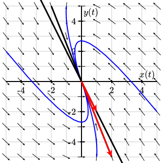
Since \(\lambda_2 - \lambda_1 \gt 0\text{,}\) the derivative, \(dy/dx\text{,}\) must approach \(\pm \infty\text{,}\) provided \(c_2 \neq 0\text{.}\) Therefore, the solutions tend towards the origin tangentially to the \(y\)-axis (Figure 3.3.7). We say that the equilibrium point for this system is a sink.
Diagram Exploration Keyboard Controls
Key Action
Enter, A Activate keyboard driven exploration
B Activate menu driven exploration
Escape Leave exploration mode
Cursor down Explore next lower level
Cursor up Explore next upper level
Cursor right Explore next element on level
Cursor left Explore previous element on level
X Toggle expert mode
W Extra details if available
Space Repeat speech
M Activate step magnification
Comma Activate direct magnification
N Deactivate magnification
Z Toggle subtitles
C Cycle contrast settings
T Monochrome colours
L Toggle language (if available)
K Kill current sound
Y Stop sound output
O Start and stop sonification
P Repeat sonification output
Figure 3.3.7. Sink phase portrait
Since \(\lambda_1 \lt \lambda_2 \lt 0\text{,}\) we say that \(\lambda_1\) is the dominant eigenvalue. The \(x\)-coordinates of the solutions approach the origin much faster than the \(y\)-coordinates.
To see what happens in the general case, suppose that \(\lambda_1 \lt \lambda_2 \lt 0\text{,}\) the eigenvectors associated with \(\lambda_1\) and \(\lambda_2\) are \((u_1, u_2)\) and \((v_1, v_2)\text{,}\) respectively. The general solution of our system is
\begin{equation*} {\mathbf x}(t) = c_1 e^{\lambda_1 t} \begin{pmatrix} u_1 \\ u_2 \end{pmatrix} + c_2 e^{\lambda_2 t} \begin{pmatrix} v_1 \\ v_2 \end{pmatrix}. \end{equation*}
The slope of a solution curve at \((x, y)\) is given by
\begin{align*} \frac{dy}{dx} & = \frac{\lambda_1 c_1 e^{\lambda_1 t} u_2 + \lambda_2 c_2 e^{\lambda_2 t} v_2} {\lambda_1 c_1 e^{\lambda_1 t} u_1 + \lambda_2 c_2 e^{\lambda_2 t} v_1}\\ & = \left( \frac{\lambda_1 c_1 e^{\lambda_1 t} u_2 + \lambda_2 c_2 e^{\lambda_2 t} v_2} {\lambda_1 c_1 e^{\lambda_1 t} u_1 + \lambda_2 c_2 e^{\lambda_2 t} v_1} \right) \frac{e^{-\lambda_2 t}}{e^{-\lambda_2 t}}\\ & = \frac{\lambda_1 c_1 e^{(\lambda_1 - \lambda_2) t} u_2 + \lambda_2 c_2 v_2} {\lambda_1 c_1 e^{(\lambda_1 - \lambda_2) t} u_1 + \lambda_2 c_2 v_1}. \end{align*}
This last expression tends toward the slope \(v_2/v_1\) of the eigenvector of \(\lambda_2\) (unless \(c_2 = 0\)). If \(c_2 = 0\text{,}\) then we have the straight-line solution corresponding to the eigenvalue \(\lambda_1\text{.}\) Hence, all the solutions for this case (except those on the straight-line belonging to the dominant eigenvalue) tend toward the origin tangentially to the straight-line solution corresponding to the weaker eigenvalue, \(\lambda_2\text{.}\)

Example 3.3.8.

Consider the system
\begin{equation*} \begin{pmatrix} x'(t) \\ y'(t) \end{pmatrix} = \begin{pmatrix} -5 \amp -2 \\ -1 \amp -4 \end{pmatrix} \begin{pmatrix} x(t) \\ y(t) \end{pmatrix}. \end{equation*}
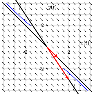
The eigenvalues of this system are \(\lambda_1 = -6\) and \(\lambda_2 = -3\) with eigenvectors \(\mathbf v_1 = (2,1 )\) and \(\mathbf v_2 = (1, -1)\text{,}\) respectively. Since the dominant eigenvalue is \(\lambda_1 = -6\text{,}\) solutions tend towards the straight-line solution containing the vector \(\mathbf v_1 = (2,1 )\) more quickly (Figure 3.3.9).
Diagram Exploration Keyboard Controls
Key Action
Enter, A Activate keyboard driven exploration
B Activate menu driven exploration
Escape Leave exploration mode
Cursor down Explore next lower level
Cursor up Explore next upper level
Cursor right Explore next element on level
Cursor left Explore previous element on level
X Toggle expert mode
W Extra details if available
Space Repeat speech
M Activate step magnification
Comma Activate direct magnification
N Deactivate magnification
Z Toggle subtitles
C Cycle contrast settings
T Monochrome colours
L Toggle language (if available)
K Kill current sound
Y Stop sound output
O Start and stop sonification
P Repeat sonification output
Figure 3.3.9. Sink phase portrait

Activity 3.3.10 Planar Systems with Two Negative Eigenvalues.

Consider the system \(d\mathbf x/dt = A \mathbf x\text{,}\) where
\begin{equation*} A = \begin{pmatrix} 6 \amp 14 \\ -4 \amp -9 \end{pmatrix} \end{equation*}

(a)

Find the eigenvalues of \(A\text{.}\) You should find distinct real eigenvalues \(\lambda\) and \(\mu\text{.}\)

(b)

Find eigenvectors \(\mathbf v_1\) and \(\mathbf v_2\) for the eigenvalues \(\lambda\) and \(\mu\text{,}\) respectively.

(c)

Find the straight-line solutions of \(d\mathbf x/dt = A \mathbf x\text{.}\) Plot the solutions in the \(xy\)-plane.

(d)

Sketch several solution curves for the system \(d\mathbf x/dt = A \mathbf x\text{.}\) What do you notice about the solution curves, especially with respect to the straight-line solutions?

(e)

Which of the two eigenvalues is the dominant eigenvalue? Why?

Subsection 3.3.3 The Case \(\lambda_1 \gt \lambda_2 \gt 0\)

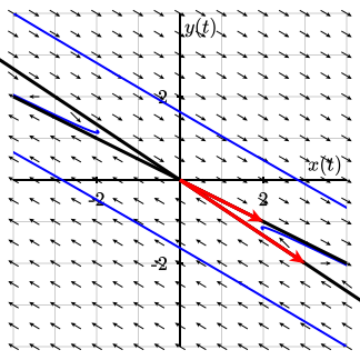
If \(\lambda_1 \gt \lambda_2 \gt 0\text{,}\) we can regard our direction field as the negative of the direction field of the previous case. The general solution and the direction field are the same, but the arrows are reversed (Figure 3.3.11). In this case, we say that the equilibrium point is a source.
Diagram Exploration Keyboard Controls
Key Action
Enter, A Activate keyboard driven exploration
B Activate menu driven exploration
Escape Leave exploration mode
Cursor down Explore next lower level
Cursor up Explore next upper level
Cursor right Explore next element on level
Cursor left Explore previous element on level
X Toggle expert mode
W Extra details if available
Space Repeat speech
M Activate step magnification
Comma Activate direct magnification
N Deactivate magnification
Z Toggle subtitles
C Cycle contrast settings
T Monochrome colours
L Toggle language (if available)
K Kill current sound
Y Stop sound output
O Start and stop sonification
P Repeat sonification output
Figure 3.3.11. Source phase portrait

Example 3.3.12.

Consider the system
\begin{equation*} \begin{pmatrix} x'(t) \\ y'(t) \end{pmatrix} = \begin{pmatrix} 4 \amp -3 \\ -1 \amp 2 \end{pmatrix} \begin{pmatrix} x(t) \\ y(t) \end{pmatrix}. \end{equation*}
The eigenvalues of this system are \(\lambda_1 = 5\) and \(\lambda_2 = 1\) with eigenvectors \(\mathbf v_1 = (3, -1)\) and \(\mathbf v_2 = (1, 1)\text{,}\) respectively. Since the dominant eigenvalue is \(\lambda_1 = 5\text{,}\) solutions are closer to the straight-line solution containing the vector \(\mathbf v_2 = (3, -1)\) more as \(t \to \infty\) (Figure 3.3.13).
Diagram Exploration Keyboard Controls
Key Action
Enter, A Activate keyboard driven exploration
B Activate menu driven exploration
Escape Leave exploration mode
Cursor down Explore next lower level
Cursor up Explore next upper level
Cursor right Explore next element on level
Cursor left Explore previous element on level
X Toggle expert mode
W Extra details if available
Space Repeat speech
M Activate step magnification
Comma Activate direct magnification
N Deactivate magnification
Z Toggle subtitles
C Cycle contrast settings
T Monochrome colours
L Toggle language (if available)
K Kill current sound
Y Stop sound output
O Start and stop sonification
P Repeat sonification output
Figure 3.3.13. Source phase portrait

Subsection 3.3.4 Important Lessons

  • Given a system of linear differential equations
    \begin{equation*} \begin{pmatrix} dx/dt \\ dy/dt \end{pmatrix} = \begin{pmatrix} a & b \\ c & d \end{pmatrix} \begin{pmatrix} x \\ y \end{pmatrix} = A \begin{pmatrix} x \\ y \end{pmatrix}, \end{equation*}
    we can use the eigenvalues of \(A\) to find and classify the solutions of the system.
  • If
    \begin{equation*} A = \begin{pmatrix} \lambda_1 & 0 \\ 0 & \lambda_2 \end{pmatrix}, \end{equation*}
    then \(A\) has two distinct real eigenvalues. The general solution to the system \({\mathbf x}' = A {\mathbf x}\) is
    \begin{equation*} {\mathbf x}(t) = \alpha e^{\lambda_1 t} \begin{pmatrix} 1 \\ 0 \end{pmatrix} + \beta e^{\lambda_2 t} \begin{pmatrix} 0 \\ 1 \end{pmatrix}. \end{equation*}
    • For the case \(\lambda_1 \lt 0 \lt \lambda_2\text{,}\) the equilibrium point of the system \({\mathbf x}' = A {\mathbf x}\) is a saddle.
    • For the case \(\lambda_1 \lt \lambda_2 \lt 0\text{,}\) the equilibrium point of the system \({\mathbf x}' = A {\mathbf x}\) is a sink.
    • For the case \(0 \lt \lambda_1 \lt \lambda_2\text{,}\) the equilibrium point of the system \({\mathbf x}' = A {\mathbf x}\) is a source.

Reading Questions 3.3.5 Reading Questions

1.

What is a stable line of solutions?

2.

For a \(2 \times 2\) linear system with distinct real eigenvalues, what are the three different possibilities for the phase plane of the system?

Exercises 3.3.6 Exercises

Phase Plane Analysis of Linear Systems with Distinct Real Eigenvalues.

For each of the linear systems \(d\mathbf x/dt = A \mathbf x\) in Exercise Group 3.3.6.1–8
  1. Find the eigenvalues of \(A\text{.}\)
  2. What is the dominant eigenvalue?
  3. Find the eigenvectors for each eigenvalue of \(A\text{.}\)
  4. What are the straight-line solutions of \(d\mathbf x/dt = A \mathbf x\text{?}\)
  5. Describe the nature of the equilibrium solution at \(\mathbf 0\text{.}\)
  6. Sketch the phase plane and several solution curves.

1.

\begin{equation*} A = \begin{pmatrix} -1 \amp 2 \\ -6 \amp 6 \end{pmatrix} \end{equation*}
Solution.
  1. The characteristic equation of \(A = \begin{pmatrix}-1 & 2 \\ -6 & 6\end{pmatrix}\) is
    \begin{align*} \det(A - \lambda I) \amp = (-1-\lambda)(6-\lambda) + 12\\ \amp = \lambda^2 - 5\lambda + 6\\ \amp = (\lambda-2)(\lambda-3) = 0, \end{align*}
    giving eigenvalues \(\lambda_1 = 2\) and \(\lambda_2 = 3\text{.}\)
  2. The dominant eigenvalue is \(\lambda_2 = 3\text{,}\) since it has the larger absolute value and governs the long-term behavior of solutions.
  3. For \(\lambda_1 = 2\text{:}\) solving \((A - 2I)\mathbf{v} = \mathbf{0}\text{,}\)
    \begin{equation*} \begin{pmatrix}-3 & 2 \\ -6 & 4\end{pmatrix} \mathbf{v} = \mathbf{0} \implies \mathbf{v}_1 = \begin{pmatrix}2\\3\end{pmatrix}. \end{equation*}
    For \(\lambda_2 = 3\text{:}\) solving \((A - 3I)\mathbf{v} = \mathbf{0}\text{,}\)
    \begin{equation*} \begin{pmatrix}-4 & 2 \\ -6 & 3\end{pmatrix} \mathbf{v} = \mathbf{0} \implies \mathbf{v}_2 = \begin{pmatrix}1\\2\end{pmatrix}. \end{equation*}
  4. The straight-line solutions of \(d\mathbf{x}/dt = A\mathbf{x}\) are
    \begin{equation*} \mathbf{x}(t) = c_1 e^{2t}\begin{pmatrix}2\\3\end{pmatrix} \qquad\text{and}\qquad \mathbf{x}(t) = c_2 e^{3t}\begin{pmatrix}1\\2\end{pmatrix}, \end{equation*}
    where \(c_1\) and \(c_2\) are arbitrary constants. The general solution is
    \begin{equation*} \mathbf{x}(t) = c_1 e^{2t}\begin{pmatrix}2\\3\end{pmatrix} + c_2 e^{3t}\begin{pmatrix}1\\2\end{pmatrix}. \end{equation*}
  5. Since both eigenvalues \(\lambda_1 = 2\) and \(\lambda_2 = 3\) are positive, all solutions (except the equilibrium itself) move away from the origin as \(t \to \infty\text{.}\) The equilibrium at \(\mathbf{0}\) is an unstable source (unstable node).
  6. Phase plane for \(d\mathbf{x}/dt = A\mathbf{x}\text{:}\)

2.

\begin{equation*} A = \begin{pmatrix} -12 \amp 30 \\ -5 \amp 13 \end{pmatrix} \end{equation*}
Solution.
  1. The characteristic equation is
    \begin{align*} \det(A-\lambda I) \amp = (-12-\lambda)(13-\lambda)+150\\ \amp = \lambda^2 - \lambda - 6\\ \amp = (\lambda-3)(\lambda+2) = 0, \end{align*}
    giving eigenvalues \(\lambda_1 = 3\) and \(\lambda_2 = -2\text{.}\)
  2. The dominant eigenvalue is \(\lambda_1 = 3\text{.}\)
  3. For \(\lambda_1 = 3\text{:}\) solving \((A-3I)\mathbf{v}=\mathbf{0}\text{,}\)
    \begin{equation*} \begin{pmatrix}-15&30\\-5&10\end{pmatrix} \mathbf{v}=\mathbf{0} \implies \mathbf{v}_1=\begin{pmatrix}2\\1\end{pmatrix}. \end{equation*}
    For \(\lambda_2 = -2\text{:}\) solving \((A+2I)\mathbf{v}=\mathbf{0}\text{,}\)
    \begin{equation*} \begin{pmatrix}-10&30\\-5&15\end{pmatrix} \mathbf{v}=\mathbf{0} \implies \mathbf{v}_2=\begin{pmatrix}3\\1\end{pmatrix}. \end{equation*}
  4. The straight-line solutions are
    \begin{equation*} \mathbf{x}(t) = c_1 e^{3t}\begin{pmatrix}2\\1\end{pmatrix} \quad\text{and}\quad \mathbf{x}(t) = c_2 e^{-2t}\begin{pmatrix}3\\1\end{pmatrix}. \end{equation*}
    The general solution is
    \begin{equation*} \mathbf{x}(t) = c_1 e^{3t}\begin{pmatrix}2\\1\end{pmatrix} + c_2 e^{-2t}\begin{pmatrix}3\\1\end{pmatrix}. \end{equation*}
  5. Since the eigenvalues \(\lambda_1 = 3\) and \(\lambda_2 = -2\) have opposite signs, the equilibrium at \(\mathbf{0}\) is an unstable saddle. Solutions on the stable manifold (along \(\mathbf{v}_2\)) approach the origin; all other solutions are eventually repelled along directions parallel to \(\mathbf{v}_1\text{.}\)

3.

\begin{equation*} A = \begin{pmatrix} -9 \amp -2 \\ 10 \amp 0 \end{pmatrix} \end{equation*}
Solution.
  1. The characteristic equation of \(A = \begin{pmatrix}-9 & -2 \\ 10 & 0\end{pmatrix}\) is
    \begin{align*} \det(A - \lambda I) \amp = (-9-\lambda)(-\lambda) + 20\\ \amp = \lambda^2 + 9\lambda + 20\\ \amp = (\lambda+4)(\lambda+5) = 0, \end{align*}
    giving eigenvalues \(\lambda_1 = -4\) and \(\lambda_2 = -5\text{.}\)
  2. The dominant eigenvalue is \(\lambda_1 = -4\text{,}\) since it has the smaller absolute value and governs the long-term behavior: as \(t \to \infty\) the \(e^{-5t}\) term decays faster, leaving the \(e^{-4t}\) term dominant.
  3. For \(\lambda_1 = -4\text{:}\) solving \((A+4I)\mathbf{v}=\mathbf{0}\text{,}\)
    \begin{equation*} \begin{pmatrix}-5&-2\\10&4\end{pmatrix} \mathbf{v}=\mathbf{0} \implies \mathbf{v}_1=\begin{pmatrix}2\\-5\end{pmatrix}. \end{equation*}
    For \(\lambda_2 = -5\text{:}\) solving \((A+5I)\mathbf{v}=\mathbf{0}\text{,}\)
    \begin{equation*} \begin{pmatrix}-4&-2\\10&5\end{pmatrix} \mathbf{v}=\mathbf{0} \implies \mathbf{v}_2=\begin{pmatrix}1\\-2\end{pmatrix}. \end{equation*}
  4. The straight-line solutions are
    \begin{equation*} \mathbf{x}(t) = c_1 e^{-4t}\begin{pmatrix}2\\-5\end{pmatrix} \quad\text{and}\quad \mathbf{x}(t) = c_2 e^{-5t}\begin{pmatrix}1\\-2\end{pmatrix}. \end{equation*}
    The general solution is
    \begin{equation*} \mathbf{x}(t) = c_1 e^{-4t}\begin{pmatrix}2\\-5\end{pmatrix} + c_2 e^{-5t}\begin{pmatrix}1\\-2\end{pmatrix}. \end{equation*}
  5. Since both eigenvalues \(\lambda_1 = -4\) and \(\lambda_2 = -5\) are negative, every solution tends to the origin as \(t \to \infty\text{.}\) The equilibrium at \(\mathbf{0}\) is a stable sink (stable node). Trajectories approach the origin tangent to the dominant eigenvector direction \(\mathbf{v}_1 = (2,-5)^T\text{.}\)

4.

\begin{equation*} A = \begin{pmatrix} 11 \amp 8 \\ -12 \amp -9 \end{pmatrix} \end{equation*}
Solution.
  1. The characteristic equation of \(A = \begin{pmatrix}11 & 8 \\ -12 & -9\end{pmatrix}\) is
    \begin{align*} \det(A - \lambda I) \amp = (11-\lambda)(-9-\lambda) + 96\\ \amp = \lambda^2 - 2\lambda - 3\\ \amp= (\lambda-3)(\lambda+1) = 0, \end{align*}
    giving eigenvalues \(\lambda_1 = 3\) and \(\lambda_2 = -1\text{.}\)
  2. The dominant eigenvalue is \(\lambda_1 = 3\text{,}\) since it has the larger absolute value and governs the long-term growth of solutions.
  3. For \(\lambda_1 = 3\text{:}\) solving \((A - 3I)\mathbf{v} = \mathbf{0}\text{,}\)
    \begin{equation*} \begin{pmatrix}8&8\\-12&-12\end{pmatrix} \mathbf{v} = \mathbf{0} \implies \mathbf{v}_1 = \begin{pmatrix}1\\-1\end{pmatrix}. \end{equation*}
    For \(\lambda_2 = -1\text{:}\) solving \((A + I)\mathbf{v} = \mathbf{0}\text{,}\)
    \begin{equation*} \begin{pmatrix}12&8\\-12&-8\end{pmatrix} \mathbf{v} = \mathbf{0} \implies \mathbf{v}_2 = \begin{pmatrix}2\\-3\end{pmatrix}. \end{equation*}
  4. The straight-line solutions are
    \begin{equation*} \mathbf{x}(t) = c_1 e^{3t}\begin{pmatrix}1\\-1\end{pmatrix} \quad\text{and}\quad \mathbf{x}(t) = c_2 e^{-t}\begin{pmatrix}2\\-3\end{pmatrix}. \end{equation*}
    The general solution is
    \begin{equation*} \mathbf{x}(t) = c_1 e^{3t}\begin{pmatrix}1\\-1\end{pmatrix} + c_2 e^{-t}\begin{pmatrix}2\\-3\end{pmatrix}. \end{equation*}
  5. Since the eigenvalues \(\lambda_1 = 3\) and \(\lambda_2 = -1\) have opposite signs, the equilibrium at \(\mathbf{0}\) is an unstable saddle. Solutions on the stable manifold (along \(\mathbf{v}_2\)) approach the origin as \(t \to \infty\text{;}\) all other solutions are eventually repelled along directions parallel to \(\mathbf{v}_1\text{.}\)

5.

\begin{equation*} A = \begin{pmatrix} 7 \amp 12 \\ -4 \amp -7 \end{pmatrix} \end{equation*}
Solution.
  1. The characteristic equation of \(A = \begin{pmatrix}7 & 12 \\ -4 & -7\end{pmatrix}\) is
    \begin{align*} \det(A - \lambda I) \amp = (7-\lambda)(-7-\lambda) + 48\\ \amp = \lambda^2 - 1\\ \amp = (\lambda-1)(\lambda+1) = 0, \end{align*}
    giving eigenvalues \(\lambda_1 = 1\) and \(\lambda_2 = -1\text{.}\)
  2. The dominant eigenvalue is \(\lambda_1 = 1\text{,}\) since it governs the long-term growth of solutions.
  3. For \(\lambda_1 = 1\text{:}\) solving \((A - I)\mathbf{v} = \mathbf{0}\text{,}\)
    \begin{equation*} \begin{pmatrix}6&12\\-4&-8\end{pmatrix} \mathbf{v} = \mathbf{0} \implies \mathbf{v}_1 = \begin{pmatrix}2\\-1\end{pmatrix}. \end{equation*}
    For \(\lambda_2 = -1\text{:}\) solving \((A + I)\mathbf{v} = \mathbf{0}\text{,}\)
    \begin{equation*} \begin{pmatrix}8&12\\-4&-6\end{pmatrix} \mathbf{v} = \mathbf{0} \implies \mathbf{v}_2 = \begin{pmatrix}3\\-2\end{pmatrix}. \end{equation*}
  4. The straight-line solutions are
    \begin{equation*} \mathbf{x}(t) = c_1 e^{t}\begin{pmatrix}2\\-1\end{pmatrix} \quad\text{and}\quad \mathbf{x}(t) = c_2 e^{-t}\begin{pmatrix}3\\-2\end{pmatrix}. \end{equation*}
    The general solution is
    \begin{equation*} \mathbf{x}(t) = c_1 e^{t}\begin{pmatrix}2\\-1\end{pmatrix} + c_2 e^{-t}\begin{pmatrix}3\\-2\end{pmatrix}. \end{equation*}
  5. Since the eigenvalues \(\lambda_1 = 1\) and \(\lambda_2 = -1\) have opposite signs, the equilibrium at \(\mathbf{0}\) is an unstable saddle. Solutions on the stable manifold (along \(\mathbf{v}_2\)) approach the origin as \(t \to \infty\text{;}\) all other solutions are eventually repelled along directions parallel to \(\mathbf{v}_1\text{.}\)

6.

\begin{equation*} A = \begin{pmatrix} 10 \amp 12 \\ -4 \amp -4 \end{pmatrix} \end{equation*}
Solution.
  1. The characteristic equation of \(A = \begin{pmatrix}10 & 12 \\ -4 & -4\end{pmatrix}\) is
    \begin{align*} \det(A - \lambda I) \amp = (10-\lambda)(-4-\lambda) + 48\\ \amp = \lambda^2 - 6\lambda + 8\\ \amp = (\lambda-2)(\lambda-4) = 0, \end{align*}
    giving eigenvalues \(\lambda_1 = 4\) and \(\lambda_2 = 2\text{.}\)
  2. The dominant eigenvalue is \(\lambda_1 = 4\text{,}\) since it has the larger value and governs the long-term behavior: as \(t \to \infty\) the \(e^{4t}\) term grows faster than \(e^{2t}\text{.}\)
  3. For \(\lambda_1 = 4\text{:}\) solving \((A - 4I)\mathbf{v} = \mathbf{0}\text{,}\)
    \begin{equation*} \begin{pmatrix}6&12\\-4&-8\end{pmatrix} \mathbf{v} = \mathbf{0} \implies \mathbf{v}_1 = \begin{pmatrix}2\\-1\end{pmatrix}. \end{equation*}
    For \(\lambda_2 = 2\text{:}\) solving \((A - 2I)\mathbf{v} = \mathbf{0}\text{,}\)
    \begin{equation*} \begin{pmatrix}8&12\\-4&-6\end{pmatrix} \mathbf{v} = \mathbf{0} \implies \mathbf{v}_2 = \begin{pmatrix}3\\-2\end{pmatrix}. \end{equation*}
  4. The straight-line solutions are
    \begin{equation*} \mathbf{x}(t) = c_1 e^{4t}\begin{pmatrix}2\\-1\end{pmatrix} \quad\text{and}\quad \mathbf{x}(t) = c_2 e^{2t}\begin{pmatrix}3\\-2\end{pmatrix}. \end{equation*}
    The general solution is
    \begin{equation*} \mathbf{x}(t) = c_1 e^{4t}\begin{pmatrix}2\\-1\end{pmatrix} + c_2 e^{2t}\begin{pmatrix}3\\-2\end{pmatrix}. \end{equation*}
  5. Since both eigenvalues \(\lambda_1 = 4\) and \(\lambda_2 = 2\) are positive, every solution (except the equilibrium itself) diverges from the origin as \(t \to \infty\text{.}\) The equilibrium at \(\mathbf{0}\) is an unstable source (unstable node). Trajectories leave the origin along directions parallel to \(\mathbf{v}_2\) and asymptotically align with \(\mathbf{v}_1\) as \(t \to \infty\text{.}\)

7.

\begin{equation*} A = \begin{pmatrix} -2 \amp -6 \\ 2 \amp 5 \end{pmatrix} \end{equation*}
Solution.
  1. The characteristic equation of \(A = \begin{pmatrix}-2 & -6 \\ 2 & 5\end{pmatrix}\) is
    \begin{align*} \det(A - \lambda I) \amp = (-2-\lambda)(5-\lambda) + 12\\ \amp = \lambda^2 - 3\lambda + 2\\ \amp = (\lambda-1)(\lambda-2) = 0, \end{align*}
    giving eigenvalues \(\lambda_1 = 2\) and \(\lambda_2 = 1\text{.}\)
  2. The dominant eigenvalue is \(\lambda_1 = 2\text{,}\) since it has the larger value and governs the long-term behavior: as \(t \to \infty\) the \(e^{2t}\) term grows faster than \(e^{t}\text{.}\)
  3. For \(\lambda_1 = 2\text{:}\) solving \((A - 2I)\mathbf{v} = \mathbf{0}\text{,}\)
    \begin{equation*} \begin{pmatrix}-4&-6\\2&3\end{pmatrix} \mathbf{v} = \mathbf{0} \implies \mathbf{v}_1 = \begin{pmatrix}3\\-2\end{pmatrix}. \end{equation*}
    For \(\lambda_2 = 1\text{:}\) solving \((A - I)\mathbf{v} = \mathbf{0}\text{,}\)
    \begin{equation*} \begin{pmatrix}-3&-6\\2&4\end{pmatrix} \mathbf{v} = \mathbf{0} \implies \mathbf{v}_2 = \begin{pmatrix}2\\-1\end{pmatrix}. \end{equation*}
  4. The straight-line solutions are
    \begin{equation*} \mathbf{x}(t) = c_1 e^{2t}\begin{pmatrix}3\\-2\end{pmatrix} \quad\text{and}\quad \mathbf{x}(t) = c_2 e^{t}\begin{pmatrix}2\\-1\end{pmatrix}. \end{equation*}
    The general solution is
    \begin{equation*} \mathbf{x}(t) = c_1 e^{2t}\begin{pmatrix}3\\-2\end{pmatrix} + c_2 e^{t}\begin{pmatrix}2\\-1\end{pmatrix}. \end{equation*}
  5. Since both eigenvalues \(\lambda_1 = 2\) and \(\lambda_2 = 1\) are positive, every solution (except the equilibrium itself) diverges from the origin as \(t \to \infty\text{.}\) The equilibrium at \(\mathbf{0}\) is an unstable source (unstable node). Trajectories leave the origin along directions parallel to \(\mathbf{v}_2\) and become asymptotically parallel to the dominant eigenvector \(\mathbf{v}_1\) as \(t \to \infty\text{.}\)

8.

\begin{equation*} A = \begin{pmatrix} -18 \amp -30 \\ 10 \amp 17 \end{pmatrix} \end{equation*}
Solution.
  1. The characteristic equation of \(A = \begin{pmatrix}-18 & -30 \\ 10 & 17\end{pmatrix}\) is
    \begin{align*} \det(A - \lambda I) \amp = (-18-\lambda)(17-\lambda) + 300\\ \amp = \lambda^2 + \lambda - 6\\ \amp = (\lambda-2)(\lambda+3) = 0, \end{align*}
    giving eigenvalues \(\lambda_1 = 2\) and \(\lambda_2 = -3\text{.}\)
  2. The dominant eigenvalue is \(\lambda_1 = 2\text{,}\) since it governs the long-term growth of solutions along the unstable manifold.
  3. For \(\lambda_1 = 2\text{:}\) solving \((A - 2I)\mathbf{v} = \mathbf{0}\text{,}\)
    \begin{equation*} \begin{pmatrix}-20&-30\\10&15\end{pmatrix} \mathbf{v} = \mathbf{0} \implies \mathbf{v}_1 = \begin{pmatrix}3\\-2\end{pmatrix}. \end{equation*}
    For \(\lambda_2 = -3\text{:}\) solving \((A + 3I)\mathbf{v} = \mathbf{0}\text{,}\)
    \begin{equation*} \begin{pmatrix}-15&-30\\10&20\end{pmatrix} \mathbf{v} = \mathbf{0} \implies \mathbf{v}_2 = \begin{pmatrix}2\\-1\end{pmatrix}. \end{equation*}
  4. The straight-line solutions are
    \begin{equation*} \mathbf{x}(t) = c_1 e^{2t}\begin{pmatrix}3\\-2\end{pmatrix} \quad\text{and}\quad \mathbf{x}(t) = c_2 e^{-3t}\begin{pmatrix}2\\-1\end{pmatrix}. \end{equation*}
    The general solution is
    \begin{equation*} \mathbf{x}(t) = c_1 e^{2t}\begin{pmatrix}3\\-2\end{pmatrix} + c_2 e^{-3t}\begin{pmatrix}2\\-1\end{pmatrix}. \end{equation*}
  5. Since the eigenvalues \(\lambda_1 = 2\) and \(\lambda_2 = -3\) have opposite signs, the equilibrium at \(\mathbf{0}\) is an unstable saddle. Solutions on the stable manifold (along \(\mathbf{v}_2\)) approach the origin as \(t \to \infty\text{;}\) all other solutions are eventually repelled along directions parallel to the unstable eigenvector \(\mathbf{v}_1\text{.}\)

9.

Solve each linear systems \(d\mathbf x/dt = A \mathbf x\) in Exercise Group 3.3.6.1–8 for the initial condition \(\mathbf x(0) = (2,2)\text{.}\)
Solution.
For each matrix we use the eigenvalues and eigenvectors found previously, write the general solution, and apply the initial condition \(\mathbf{x}(0) = (2,2)^T\text{.}\)
Matrix 1: \(A = \begin{pmatrix}-1&2\\-6&6\end{pmatrix}\text{,}\) \(\lambda_1=2\text{,}\) \(\mathbf{v}_1=(2,3)^T\text{,}\) \(\lambda_2=3\text{,}\) \(\mathbf{v}_2=(1,2)^T\text{.}\) The general solution is
\begin{equation*} \mathbf{x}(t) = c_1 e^{2t}\begin{pmatrix}2\\3\end{pmatrix} + c_2 e^{3t}\begin{pmatrix}1\\2\end{pmatrix}. \end{equation*}
Applying \(\mathbf{x}(0)=(2,2)^T\text{:}\)
\begin{align*} 2c_1 + c_2 &= 2,\\ 3c_1 + 2c_2 &= 2. \end{align*}
Solving gives \(c_1 = 2\) and \(c_2 = -2\text{,}\) so
\begin{equation*} \mathbf{x}(t) = 2e^{2t}\begin{pmatrix}2\\3\end{pmatrix} - 2e^{3t}\begin{pmatrix}1\\2\end{pmatrix}. \end{equation*}
Matrix 2: \(A = \begin{pmatrix}-12&30\\-5&13\end{pmatrix}\text{,}\) \(\lambda_1=3\text{,}\) \(\mathbf{v}_1=(2,1)^T\text{,}\) \(\lambda_2=-2\text{,}\) \(\mathbf{v}_2=(3,1)^T\text{.}\) The general solution is
\begin{equation*} \mathbf{x}(t) = c_1 e^{3t}\begin{pmatrix}2\\1\end{pmatrix} + c_2 e^{-2t}\begin{pmatrix}3\\1\end{pmatrix}. \end{equation*}
Applying \(\mathbf{x}(0)=(2,2)^T\text{:}\)
\begin{align*} 2c_1 + 3c_2 &= 2,\\ c_1 + c_2 &= 2. \end{align*}
Solving gives \(c_1 = 4\) and \(c_2 = -2\text{,}\) so
\begin{equation*} \mathbf{x}(t) = 4e^{3t}\begin{pmatrix}2\\1\end{pmatrix} - 2e^{-2t}\begin{pmatrix}3\\1\end{pmatrix}. \end{equation*}
Matrix 3: \(A = \begin{pmatrix}-9&-2\\10&0\end{pmatrix}\text{,}\) \(\lambda_1=-4\text{,}\) \(\mathbf{v}_1=(2,-5)^T\text{,}\) \(\lambda_2=-5\text{,}\) \(\mathbf{v}_2=(1,-2)^T\text{.}\) The general solution is
\begin{equation*} \mathbf{x}(t) = c_1 e^{-4t}\begin{pmatrix}2\\-5\end{pmatrix} + c_2 e^{-5t}\begin{pmatrix}1\\-2\end{pmatrix}. \end{equation*}
Applying \(\mathbf{x}(0)=(2,2)^T\text{:}\)
\begin{align*} 2c_1 + c_2 &= 2,\\ -5c_1 - 2c_2 &= 2. \end{align*}
Solving gives \(c_1 = -6\) and \(c_2 = 14\text{,}\) so
\begin{equation*} \mathbf{x}(t) = -6e^{-4t}\begin{pmatrix}2\\-5\end{pmatrix} + 14e^{-5t}\begin{pmatrix}1\\-2\end{pmatrix}. \end{equation*}
Matrix 4: \(A = \begin{pmatrix}11&8\\-12&-9\end{pmatrix}\text{,}\) \(\lambda_1=3\text{,}\) \(\mathbf{v}_1=(1,-1)^T\text{,}\) \(\lambda_2=-1\text{,}\) \(\mathbf{v}_2=(2,-3)^T\text{.}\) The general solution is
\begin{equation*} \mathbf{x}(t) = c_1 e^{3t}\begin{pmatrix}1\\-1\end{pmatrix} + c_2 e^{-t}\begin{pmatrix}2\\-3\end{pmatrix}. \end{equation*}
Applying \(\mathbf{x}(0)=(2,2)^T\text{:}\)
\begin{align*} c_1 + 2c_2 &= 2,\\ -c_1 - 3c_2 &= 2. \end{align*}
Solving gives \(c_1 = 10\) and \(c_2 = -4\text{,}\) so
\begin{equation*} \mathbf{x}(t) = 10e^{3t}\begin{pmatrix}1\\-1\end{pmatrix} - 4e^{-t}\begin{pmatrix}2\\-3\end{pmatrix}. \end{equation*}
Matrix 5: \(A = \begin{pmatrix}7&12\\-4&-7\end{pmatrix}\text{,}\) \(\lambda_1=1\text{,}\) \(\mathbf{v}_1=(2,-1)^T\text{,}\) \(\lambda_2=-1\text{,}\) \(\mathbf{v}_2=(3,-2)^T\text{.}\) The general solution is
\begin{equation*} \mathbf{x}(t) = c_1 e^{t}\begin{pmatrix}2\\-1\end{pmatrix} + c_2 e^{-t}\begin{pmatrix}3\\-2\end{pmatrix}. \end{equation*}
Applying \(\mathbf{x}(0)=(2,2)^T\text{:}\)
\begin{align*} 2c_1 + 3c_2 &= 2,\\ -c_1 - 2c_2 &= 2. \end{align*}
Solving gives \(c_1 = 10\) and \(c_2 = -6\text{,}\) so
\begin{equation*} \mathbf{x}(t) = 10e^{t}\begin{pmatrix}2\\-1\end{pmatrix} - 6e^{-t}\begin{pmatrix}3\\-2\end{pmatrix}. \end{equation*}
Matrix 6: \(A = \begin{pmatrix}10&12\\-4&-4\end{pmatrix}\text{,}\) \(\lambda_1=4\text{,}\) \(\mathbf{v}_1=(2,-1)^T\text{,}\) \(\lambda_2=2\text{,}\) \(\mathbf{v}_2=(3,-2)^T\text{.}\) The general solution is
\begin{equation*} \mathbf{x}(t) = c_1 e^{4t}\begin{pmatrix}2\\-1\end{pmatrix} + c_2 e^{2t}\begin{pmatrix}3\\-2\end{pmatrix}. \end{equation*}
Applying \(\mathbf{x}(0)=(2,2)^T\text{:}\)
\begin{align*} 2c_1 + 3c_2 &= 2,\\ -c_1 - 2c_2 &= 2. \end{align*}
Solving gives \(c_1 = 10\) and \(c_2 = -6\text{,}\) so
\begin{equation*} \mathbf{x}(t) = 10e^{4t}\begin{pmatrix}2\\-1\end{pmatrix} - 6e^{2t}\begin{pmatrix}3\\-2\end{pmatrix}. \end{equation*}
Matrix 7: \(A = \begin{pmatrix}-2&-6\\2&5\end{pmatrix}\text{,}\) \(\lambda_1=2\text{,}\) \(\mathbf{v}_1=(3,-2)^T\text{,}\) \(\lambda_2=1\text{,}\) \(\mathbf{v}_2=(2,-1)^T\text{.}\) The general solution is
\begin{equation*} \mathbf{x}(t) = c_1 e^{2t}\begin{pmatrix}3\\-2\end{pmatrix} + c_2 e^{t}\begin{pmatrix}2\\-1\end{pmatrix}. \end{equation*}
Applying \(\mathbf{x}(0)=(2,2)^T\text{:}\)
\begin{align*} 3c_1 + 2c_2 &= 2,\\ -2c_1 - c_2 &= 2. \end{align*}
Solving gives \(c_1 = -6\) and \(c_2 = 10\text{,}\) so
\begin{equation*} \mathbf{x}(t) = -6e^{2t}\begin{pmatrix}3\\-2\end{pmatrix} + 10e^{t}\begin{pmatrix}2\\-1\end{pmatrix}. \end{equation*}
Matrix 8: \(A = \begin{pmatrix}-18&-30\\10&17\end{pmatrix}\text{,}\) \(\lambda_1=2\text{,}\) \(\mathbf{v}_1=(3,-2)^T\text{,}\) \(\lambda_2=-3\text{,}\) \(\mathbf{v}_2=(2,-1)^T\text{.}\) The general solution is
\begin{equation*} \mathbf{x}(t) = c_1 e^{2t}\begin{pmatrix}3\\-2\end{pmatrix} + c_2 e^{-3t}\begin{pmatrix}2\\-1\end{pmatrix}. \end{equation*}
Applying \(\mathbf{x}(0)=(2,2)^T\text{:}\)
\begin{align*} 3c_1 + 2c_2 &= 2,\\ -2c_1 - c_2 &= 2. \end{align*}
Solving gives \(c_1 = -6\) and \(c_2 = 10\text{,}\) so
\begin{equation*} \mathbf{x}(t) = -6e^{2t}\begin{pmatrix}3\\-2\end{pmatrix} + 10e^{-3t}\begin{pmatrix}2\\-1\end{pmatrix}. \end{equation*}
10.

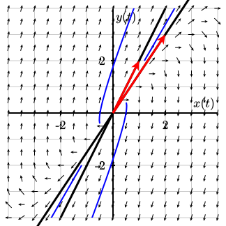
Consider the linear system \(d \mathbf x/dt = A \mathbf x\text{,}\) where
\begin{equation*} A = \begin{pmatrix} 3 \amp 2 \\ 3 \amp -2 \end{pmatrix}. \end{equation*}
Suppose the initial conditions for the solution curve are \(x(0) = 1\) and \(y(0) = 1\text{.}\) We can use the following Sage code to plot the phase portrait of this system, including the straight-line solutions and a solution curve.
Use Sage to graph the direction field for the system linear systems \(d\mathbf x/dt = A \mathbf x\) in Exercise Group 3.3.6.1–8. Plot a solution curve for the initial condition \(\mathbf x(0) = (2,2)\text{.}\) Be sure to show the corresponding straight-line solutions on your graph.
You have attempted of activities on this page.