Integration using Computer Algebra

Section 7.5 Integration using Computer Algebra

Recall that the fundamental theorem of calculus states that if $F(x)$ is a function with its derivative equal to $f(x)$ on the region $a \leq x \leq b\text{,}$ then $\int_a^b f(x)\,dx=F(b)-F(a)\text{.}$ We say $\int_a^b f(x)\,dx$ is the definite integral of $f(x)$ from $a$ to $b\text{.}$ If $f(x)$ is a derivative of $F(x)\text{,}$ then $F(x)$ is an anti-derivative of $f(x)\text{,}$ and any anti-derivative of $f(x)$ has the form $F(x) + c\text{,}$ for some constant $c\text{.}$ We use the symbol $\int f(x)\,dx\text{,}$ without limits of integration, for the indefinite integral.

In Section 7.1 we looked at approximating definite integrals with a Riemann sum that added up the area of a bunch of rectangles. In Section 7.2 we saw that the fundamental theorem of calculus lets us use an antiderivative or indefinite integral to evaluate a definite integral. In Section 7.3–7.4 we saw how to compute indefinite integrals by hand for a limited number of functions. In this section, we will look at how to use computer software at a web site to find antiderivatives.

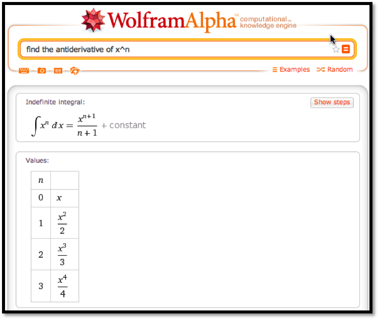
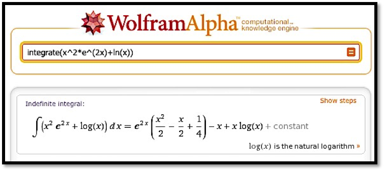
We start with Wolfram|Alpha, available at http://www.wolframalpha.com. We can give Wolfram|Alpha the question we want solved in plain English. In our case we would like to find the antiderivative of $x^n$ with respect to $x\text{.}$

The Alpha provides an answer.

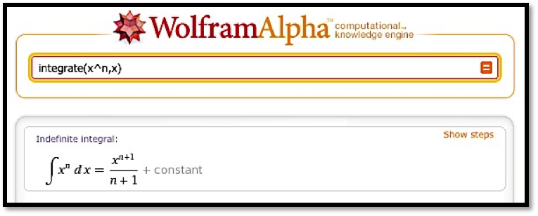
Note that the response tells us the question the Wolfram|Alpha is answering. That helps us check that we have been properly understood. We may find it useful to give a formula without the extra words.

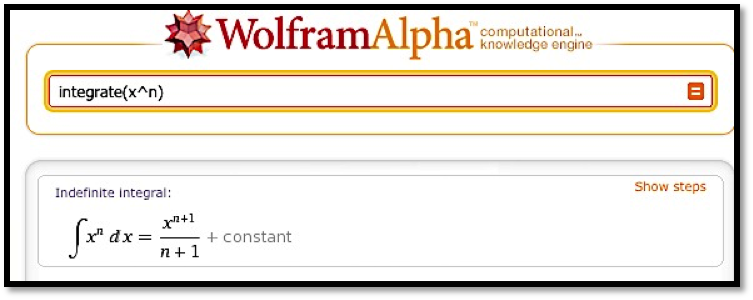
The interface is fairly robust. It understands the convention that the variable for math problems is typically $x\text{,}$ so it will generally guess that $x$ is our variable if we don’t specify the variable with respect to which we are integrating.

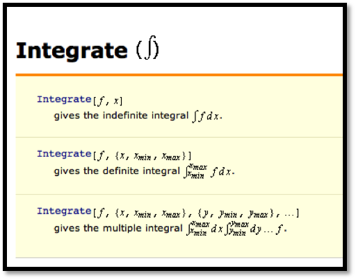
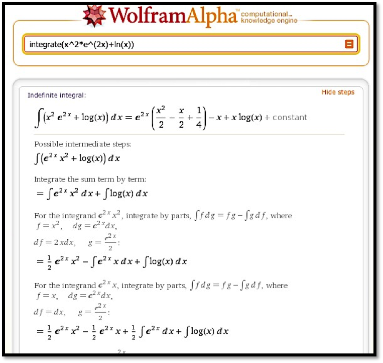
It is worth noting that Wolfram|Alpha is connected with Mathematica, so it will understand questions in Mathematica syntax. On the right side to the screen there is a link for related links. In particular, there will be a link for the related command in Mathematica.

Following that link gives more information on the syntax of the Mathematica command. We generally don’t need to know the syntax, but it is useful if we want to use specific options.

We should note that Wolfram|Alpha will easily find antiderivatives that we would find very hard to do or beyond the scope of this class.

The output also has a link for showing steps on complicated problems.

The show steps link only works on the paid version of Alpha. However we can find other tools by searching for integral calculator. Such a search reveals Symbolab, https://www.symbolab.com/solver/definite-integral-calculator, which we also used in Chapter 4.

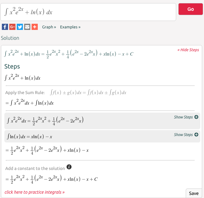
In Chapter 4, we found a derivative calculator. Similarly we can find an integral calculator (http://www.integral-calculator.com/) that will show steps. For problems of at the level of difficulty we have been doing, Wolfram|Alpha also produces plots of the integral.

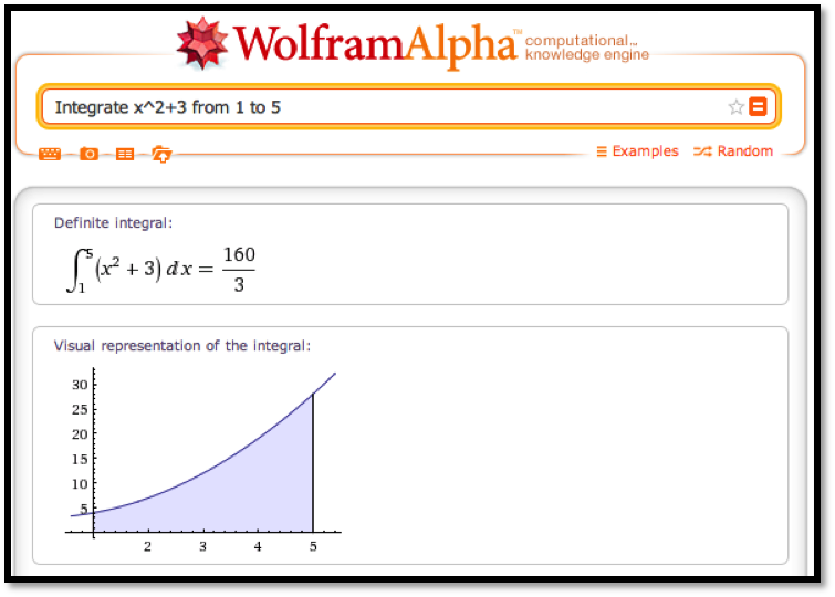
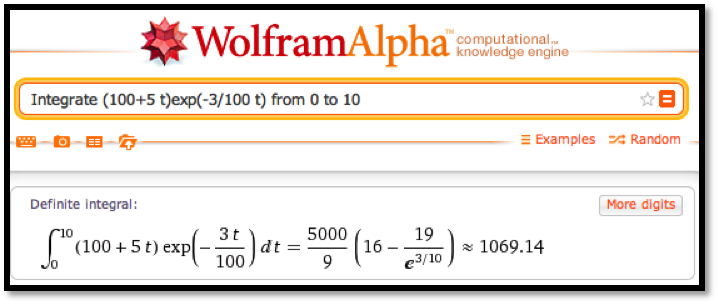
Subsection 7.5.1 Definite integrals

One of the reasons we wanted to find antiderivatives was to be able to use them to evaluate definite integrals. We can ask Wolfram|Alpha for the definite integral directly. In that case, Wolfram|Alpha will give the numeric answer and will also produce the relevant graph. (Symbolab will also do definite integrals.)

This is particularly useful when finding the antiderivative is beyond the scope of this course. Consider for example if we want to find the area under a portion of a curve that has the shape of a normal curve.

Another example when we can easily set up integrals we cannot solve by hand occurs when we are trying to find the current value of a revenue stream. A value, $V\text{,}$ that we get $t$ years in the future, has a present value of $V \exp(-r t)$ where $r$ is an investment return rate. Thus the current value of a revenue stream, $V(t)\text{,}$ from time $a$ to time $b\text{,}$ is $\int_a^b V(t)*e^{(-r*t)} dt\text{.}$ However we only have a rule for finding the antiderivative when $V(t)$ is either a constant or exponential function. With a CAS program it is straightforward to compute such integrals for a broad range of value stream functions.

If you are going to use Wolfram|Alpha in doing work, you should realize that the terms of use of the site require you to appropriately cite Wolfram|Alpha. (This is standard academic procedure.) Your citation should include that date that you got your answer from the site. The results above were obtained on Feb 29, 2012.

In business situations, we are rarely asked to simply find an integral. Instead, finding an integral is generally part of a larger problem. Thus we often use CAS for part of a problem.

Subsection 7.5.2 Initial value problems

We often want to choose a particular antiderivative of a function. We typically do this when we have the value of the antiderivative for some value. We simply plug that value into the general antiderivative and solve for $C\text{.}$

Example 7.5.1. Finding the antiderivative, then the constant.

The rate of change profit with respect to quantity is given by $P'(q)=-q^2+5q+50$ and the break-even point occurs when $q=5\text{.}$ Find the formula for profit as a function of $q\text{.}$ Find the maximum profit.

Solution.

We can do this by putting together things we have already done. First we use Wolfram|Alpha to find an antiderivative.

Thus we know $P(q)=\frac{1q^3}{3}+\frac{5q^2}{2}+50q+C$ for some constant $C\text{.}$ We also know $P(5)=0\text{.}$

Thus, $0=P(5)=\frac{5^3}{3}+\frac{5*5^2}{2}+50*5+C\text{,}$ or $--C=\frac{5^3}{3}+\frac{5*5^2}{2}+50*5\text{.}$

Using Excel, we now plug the function, without the $C\text{,}$ into Excel and evaluate at $q=5\text{.}$

We make $C$ the negative of our answer and modify our function accordingly. We now use solver to maximize the function.

Thus the maximum profit is $145.83, and it occurs when $q=10\text{.}$

Example 7.5.2. The previous example in one step.

The rate of change profit with respect to quantity is given by $P' (q)=-q^2+5q+50$ and the break-even point occurs when $q=5\text{.}$ Find the formula for profit as a function of $q\text{.}$ Find the maximum profit.

Solution.

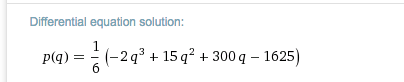
We can also do this with Wolfram|Alpha bysetting up the boundary value problem. We give the alpha bot the derivative we want integrated and the fixed value of the original function. (Notice that the answer does not include a $+C\text{,}$ since we have computed a particular constant.)

We then ask Alpha to maximize the function.

This gives the same answer of $145.83.

This first example could easily have been done by hand. We can repeat the process with an example that could not be easily been by hand.

Example 7.5.3. A more complicated initial value problem.

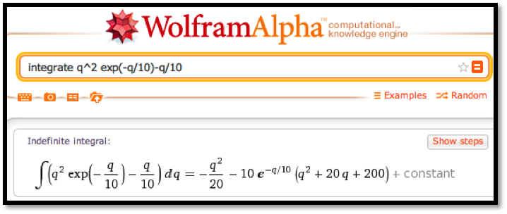
The rate of change of profit with respect to quantity is given by $P' (q)=q^2 \exp(-q/10)-q/10$ and a break-even point occurs when $q = 5\text{.}$ Find the formula for profit as a function of $q\text{.}$ Find the maximum profit.

Solution.

In structure, this example is very similar to the first example. However, where in the first example, the function would have been easy to do by hand, in this case, the problem is very hard to do by hand. We use Wolfram/Alpha to find the antiderivative.

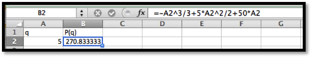
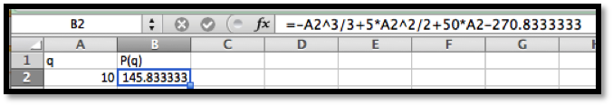
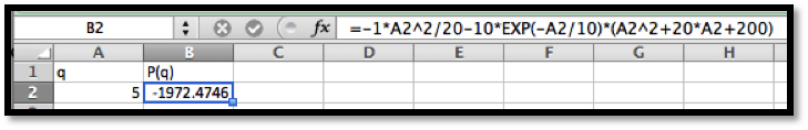
\begin{equation*} P(q) = \exp(-q/10)*(-10*q^2-200*q-2000)-q^2/20+C\text{.} \end{equation*}

We then use Excel to find $C\text{,}$ noting that if we use $P(q)$ without the $C\text{,}$ then $C$ is the value of $-P(5) = 1972.474\text{.}$

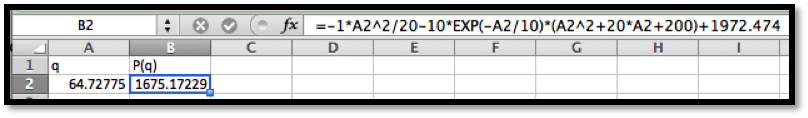
We plug in 5 and note $P(5) = 0 = C-1972.474\text{,}$ thus $C = 1972.474\text{.}$ We use solver to maximize and find the maximum profit of $1675.17 occurs at $q=64.72775\text{.}$

Subsection 7.5.3 Riemann Sums

We can also use Alpha to do Riemann sums. We need to give a starting and ending point and the number of intervals.

Example 7.5.4. Riemann sums with Wolfram|Alpha.

Find the current value of a revenue stream $V(t)=2000+5t$ for 10 years with an investment rate of $r=1.03\text{,}$ assuming payments are made daily.

Solution.

We approximate the current value with the integral

\begin{equation*} \text{CurrentValue}=\int_{\text{start}}^{\text{stop}} r^{-t} V(t)dt= \int_0^{10} 1.03^{-t} (2000+5t)\,dt\text{.} \end{equation*}

What we really want is the Riemann sum with one interval per day. Over 10 years we have 3652 days.

If we assume payments start at the beginning of the first day, we would use the left endpoint method.

Exercises 7.5.4 Exercises: Integration using Computer Algebra Problems

1. Reading check, Integration Using Computer Algebra.

This question checks your reading comprehension of the material is section 7.5, Integration Using Computer Algebra, of Business Calculus with Excel. Based on your reading, select all statements that are correct. There may be more than one correct answer. The statements may appear in what seems to be a random order.

The section uses Symbolab as a computer algebra system that will do integration.
The section uses GeoGebra as a computer algebra system that will do integration.
Wolfram|Alpha will also do definite integrals.
The computer algebra systems used in this section cannot do Riemann sums.
In initial value problems, we have to solve for the value of the integration constant $C\text{.}$
The section uses Wolfram|Alpha as a computer algebra system that will do integration.
None of the above

Answer.

$\text{A, C, E, F}$

Exercise Group.

Find the antiderivative of the given function.

2.

\begin{equation*} f(x)=x \ln(x)\text{.} \end{equation*}

Solution.

\begin{equation*} \int x \ln(x)dx=\frac{1}{4} x^{2}(2\ln(x)-1) +c\text{.} \end{equation*}

3.

\begin{equation*} f(t)=e^{.07t} (-t^2+3t+5)\text{.} \end{equation*}

4.

\begin{equation*} f(t)=t^2 e^(-0.06t)\text{.} \end{equation*}

Solution.

\begin{equation*} \int t^2 e^{-0.06 t} dt= e^{-0.06t} (-9259.26 - 555.556 t - 16.6667 t^2)+c\text{.} \end{equation*}

5.

\begin{equation*} f(x)=\ln(x)\text{.} \end{equation*}

6.

\begin{equation*} f(t)=(t+1) e^{-0.06t}\text{.} \end{equation*}

Solution.

\begin{equation*} \int (t+1) e^{-0.06t}\,dt =e^(-0.06t) (-294.444 - 16.6667 t)+c\text{.} \end{equation*}

7.

\begin{equation*} f(x)=\frac{1}{(1+2x)(3+x)(5+6x) }\text{.} \end{equation*}

8.

\begin{equation*} f(x)=\frac{1}{\sqrt{1+x^2}}\text{.} \end{equation*}

Solution.

\begin{equation*} \int \frac{1}{\sqrt{1+x^2}}\,dx= \sinh^{-1}(x)+c\text{.} \end{equation*}

9.

\begin{equation*} f(x)=\frac{1}{(3+2x)^2} \text{.} \end{equation*}

10.

\begin{equation*} f(x)=\frac{5}{9+x^2 }\text{.} \end{equation*}

Solution.

\begin{equation*} \int \frac{5}{9+x^2 }\,dx = \left(\frac{5}{3}\right)\tan^{-1}\left(\frac{x}{3}\right)+c\text{.} \end{equation*}

11.

\begin{equation*} f(x)=\frac{1}{(5x+4)^2 (7x+9)}\text{.} \end{equation*}

Exercise Group.

Evaluate the definite integral.

12.

\begin{equation*} \int_0^{10} t^2 e^{-0.06t} dt \text{.} \end{equation*}

Solution.

\begin{equation*} \int_0^{10} t^2 e^{-0.06t} dt \approx 214.03\text{.} \end{equation*}

13.

\begin{equation*} \int_1^{10}\frac{dt}{t} \text{.} \end{equation*}

14.

\begin{equation*} \int_1^8(x-1)(x-8) dx\text{.} \end{equation*}

Solution.

\begin{equation*} \int_1^8(x-1)(x-8) dx \approx -57.167\text{.} \end{equation*}

15.

\begin{equation*} \int_0^{10}t^2 e^{.05(10-t)} dt \text{.} \end{equation*}

16.

\begin{equation*} \int_0^2 e^{-x^2} dx\text{.} \end{equation*}

Solution.

\begin{equation*} \int_0^2 e^{-x^2} dx \approx 0.882081\text{.} \end{equation*}

17.

\begin{equation*} \int_9^{16} \frac{1}{\sqrt{2\pi}} e^{-(x-10)^2} dx \text{.} \end{equation*}

Exercise Group.

Do the initial value problem.

18.

\begin{equation*} P' (q)=-q^2+3q+5\text{ and }P(3)=5.\text{ Find } P(q)\text{.} \end{equation*}

Solution.

\begin{equation*} P(q)=\frac{1}{6} (-2q^3+9q^2+30q-87)\text{.} \end{equation*}

19.

\begin{equation*} F' (t)=t^2 e^{-0.1t} \text{ and } F(10)=2. \text{ Find } F(t)\text{.} \end{equation*}

20.

\begin{equation*} P' (q)=\sqrt{q^2+5q+7} \text{ and } P(0)=7. \text{ Find } P(q)\text{.} \end{equation*}

Solution.

\begin{align*} P(q) \amp = (56 - 50 \sqrt{157} + (4q+10) \sqrt{7 + 5 q + q^2} \\ \amp - 3 \sinh^{-1}\left(\frac{25}{\sqrt{3}}\right)+ 3 \sinh^{-1}\left(\frac{5 + 2 q}{\sqrt{3}}\right))/8\text{.} \end{align*}

21.

\begin{equation*} P' (q)=-(q^2+2q+3)^2 \text{ and } P(10)=-7. \text{ Find } P(q)\text{.} \end{equation*}

22.

I have an investment that produces income at a rate of $P(t)=5000+100t\text{.}$ I assume the present value of an asset decreases continuously at a rate of 2% per year for the length of time I have to wait for the asset. What is the present value of the first 7 years of return from my investment?

Solution.

\begin{equation*} \int_0^7(5000+100t) (.98)^t dt\approx 34868.6\text{.} \end{equation*}

23.

My oil well is producing revenue at a rate of $P(t)=5000(0.09^t)\text{.}$ I assume the present value of an asset decreases continuously at a rate of 3% per year for the length of time I have to wait for the asset. What is the present value of the first 10 years of return from my investment?

24.

The rate of marginal profit is $MP(q)=100-12\ln(q)$ and a break-even point occurs at $q=100\text{.}$ Find the quantity that produces the most profit and the amount of profit generated at that point.

Solution.

We have maximal profit when $MP(q)=0\text{,}$ or when $q=e^8=2981\text{.}$ Using WolframAlpha to solve the initial value problem we get

\begin{align*} P(q)\amp =16(7q-700+75ln(100))-12q ln(q)\\ P(2981)\amp = 16(7*2981-700+75ln(100))-12*2981 ln(2981)=42021.7\text{.} \end{align*}

25.

Our marginal cost function is $MC(q)=10q \ln(q)$ and the startup costs are $23,000. Produce a cost function.

You have attempted of activities on this page.

Prev Top Next