
Business Calculus with Excel

Section 6.3 Critical Points and Extrema

Subsection 6.3.1 Critical Points

With functions of one variable we were interested in places where the derivative is zero, since they made candidate points for the maximum or minimum of a function. If the derivative is not zero, we have a direction that is downhill and moving a little in that direction gives a lower value of the function. Similarly, with functions of two variables we can only find a minimum or maximum for a function if both partial derivatives are 0 at the same time. Such points are called critical points.
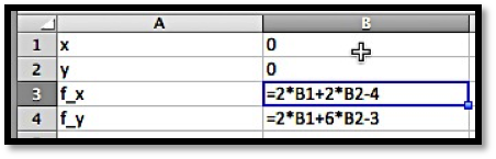
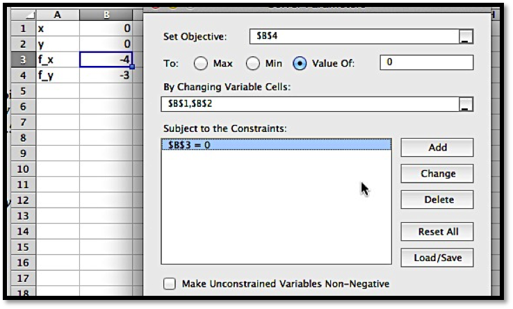
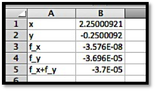
The point \((a,b)\) is a critical point for the multivariable function \(f(x,y)\text{,}\) if both partial derivatives are 0 at the same time.
In other words,
\begin{equation*} \frac{\partial }{\partial x} f(x,y)|_{x=a,y=b}=0 \end{equation*}
and
\begin{equation*} \frac{\partial }{\partial y} f(x,y)|_{x=a,y=b}=0\text{.} \end{equation*}

Example 6.3.1. Finding a Local Minimum of a Function.

Figure 6.3.2. Video of finding local minimum
Use the partial derivatives of \(f(x,y)=x^2+ 2xy+3y^2-4x-3y\) to find the minimum of the graph.
Solution.
Critical Point by Algebra
In the previous section, we already computed
\begin{align*} \frac{\partial }{\partial x} f(x,y) \amp = 2x+2y-4\\ \frac{\partial }{\partial y} f(x,y) \amp = 2x+6y-3\text{.} \end{align*}
We need to find the places where both partial derivatives are 0. With this simple system, I can solve this system algebraically and find the only critical point is \((9/4, -1/4)\text{.}\)
\begin{align*} 0 \amp = 2x+2y-4\\ 0 \amp = 2x+6y-3\text{.} \end{align*}
Subtract the equations to eliminate \(x\text{:}\)
\begin{equation*} 0=0-4y-1\text{.} \end{equation*}
Solve for \(y\text{:}\)
\begin{align*} 4y \amp = -1\\ y \amp = -1/4\text{.} \end{align*}
Substitute back and solve for \(x\text{:}\)
\begin{align*} 0 \amp = 2x+2(-1/4)-4\\ 2x \amp = 9/2\\ x \amp =9/4\text{.} \end{align*}
Critical Point by Solver
If the partials are more complicated, I will want to find the critical points another way. I can find the point with Solver.
Figure 6.3.3. Critical point setup
To get solver to set both partials to 0 at the same time, I ask it to solve for \(f_y=0\text{,}\) while setting \(f_x=0\) as a constraint. Make sure to uncheck the box that makes unconstrained variables non-negative.
Figure 6.3.4. Critical point setup
This finds our critical point within our error tolerance.
Critical Point by CAS
We can also use Wolfram|Alpha to find the solution to our system of equations.
Determining the Critical Point is a Minimum
We thus get a critical point at \((9/4,-1/4)\) with any of the three methods of solving for both partial derivatives being zero at the same time. Once we have a critical point we want to determine if it is a maximum, minimum, or something else. The easiest way is to look at the graph near the critical point.
It is clear from the graph that this critical point is a local minimum.
It is easy to see that \(f(x,y)=x^2+y^2\) has a critical point at \((0,0)\) and that that point is a minimum for the function. Similarly, \(f(x,y)=-x^2-y^2\) has a critical point at \((0,0)\) and that that point is a maximum for the function. For some functions, like \(f(x,y)=x^2-y^2\text{,}\) which has a critical point at \((0,0)\text{,}\) we can have a maximum in one direction and a minimum in another direction. Such a point is called a saddle point. We note that we can have a saddle point even if the \(x\) and \(y\) slice curves both indicate a minimum.

Example 6.3.5. A Saddle Point at a Minimum on Both Axes.

Figure 6.3.6. Video presentation of this example
Show that \(f(x,y)=x^2-3xy+y^2\) has a critical point at \((0,0)\text{,}\) which is a minimum of both slice curves, but is not a local minimum.
Solution.
We look at the two partial derivatives, and notice they are both zero at the origin.
\begin{align*} \frac{\partial }{\partial x} f(x,y) \amp = 2x-3y\\ \frac{\partial }{\partial x} f(x,y) \amp = -3x+2y\text{.} \end{align*}
We then see that both slice curves are parabolas that bend up, with a minimum at 0.
\begin{align*} f(x,0) \amp = x^2\\ f(0,y) \amp = y^2\text{.} \end{align*}
However if we take the slice with \(x=y\text{,}\) we get a parabola bending down, so we don’t have a minimum.
\begin{equation*} f(x,-x)=x^2-3x x+x^2=-x^2\text{.} \end{equation*}
Looking at the graph, we see that this graph does not have a minimum.

Subsection 6.3.2 Second Partial Derivatives

With only first derivatives, we can just find the critical points. To check if a critical point is maximum, a minimum, or a saddle point, using only the first derivative, the best method is to look at a graph to determine the kind of critical point. For some applications we want to categorize the critical points symbolically.
With functions of one variable we used the second derivative to test if a critical point was a maximum or minimum. In the two variable case we need to define the second derivatives and use them to define the discriminant of a function to test if a critical point is a minimum, maximum, or saddle point. We first need to define second partial derivatives.

Second partials.

\begin{equation*} f_{ab}=(f_a )_b=\frac{\partial}{\partial b}(\frac{\partial}{\partial a} f)\text{.} \end{equation*}
Note that \(f_{xx}\) is simply the old second derivative of the curve \(f(x,y_0)\) and \(f_{yy}\) is simply the old second derivative of the curve \(f(x_0,y)\text{.}\) For functions with continuous second partial derivatives, the mixed partials, \(f_{yx}\) and \(f_{xy}\) are the same.

Example 6.3.7. Finding Second Partial Derivatives.

Find the second partial derivatives of
\begin{equation*} f(x,y)=x^2+ 3xy+5y^3-7x-11y\text{.} \end{equation*}
Solution.
We start by computing the first partial derivatives.
\begin{align*} f_x \amp = \frac{\partial}{\partial x} f(x,y)=2x+3y-7\\ f_y \amp = \frac{\partial}{\partial y} f(x,y)=3x+15y^2-11\text{.} \end{align*}
Then we compute the second partial derivatives.
\begin{align*} f_{xx} \amp = \frac{\partial}{\partial x} f_x=2\\ f_{xy} \amp = \frac{\partial}{\partial y} f_x=3\\ f_{yx} \amp = \frac{\partial}{\partial x} f_y=3\\ f_{yy} \amp = \frac{\partial}{\partial y} f_y=30y\text{.} \end{align*}
As expected, the mixed partials are the same.

Subsection 6.3.3 Using the Discriminant to Test Critical Points

To test if a critical point is a maximum, minimum, or saddle point we compute the discriminant of the function.

Discriminant.

\begin{equation*} D(f(x,y))=f_{xx} f_{yy}-f_{xy}^2\text{.} \end{equation*}

Example 6.3.8. Finding the Discriminant of a Function.

Find the discriminant of
\begin{equation*} f(x,y)=x^2+ 3xy+5y^3-7x-11y\text{.} \end{equation*}
Solution.
We have already computed the second partial derivatives.
\begin{equation*} f_{xx}=2,\quad f_{xy}=3,\quad f_{yy}=30y\text{.} \end{equation*}
Substituting into the formula,
\begin{equation*} D=(2)(30y)-3^2=60y-9\text{.} \end{equation*}

Discriminant test.

Let \((a,b)\) be a critical point of \(f(x,y)\text{.}\)
If \(D(a,b)>0\) and \(f_{xx} (a,b)>0\) then \((a,b)\) is a local minimum of \(f(x,y)\text{.}\)
If \(D(a,b)>0 \) and \(f_{xx} (a,b)\lt 0\) then \((a,b)\) is a local maximum of \(f(x,y)\text{.}\)
If \(D(a,b)\lt 0\) then \((a,b)\) is a saddle point of \(f(x,y)\text{.}\)
If \(D(a,b)=0\) we do not have enough information to classify the point.

Example 6.3.9. Using the Discriminant to Classify Critical Points.

Based on the information given, classify each of the following points as a local maximum, local minimum, saddle point, not a critical point, or not enough information to classify.
p \({f_x}\) \({f_y}\) \(f_{xx}\) \(f_{xy}\) \(f_{yy}\)
A 0 0 0 0 1
B 0 1 3 2 4
C 1 0 0 2 3
D 0 0 1 2 0
E 0 0 -1 2 3
F 0 0 -3 1 -2
G 0 0 3 3 3
Solution.
We need to compute the discriminant and apply the test.
p \(f_x\) \(f_y\) \(f_{xx}\) \(f_{xy}\) \(f_{yy}\) Discriminant Classification
A 0 0 0 0 1 0 Not enough information
B 0 1 3 2 4 8 Not a critical point
C 1 0 0 2 3 -4 Not a critical point
D 0 0 1 2 0 -4 Saddle point
E 0 0 -1 2 3 -7 Saddle point
F 0 0 -3 1 -2 5 Maximum
G 0 0 3 3 3 0 Not enough information

Example 6.3.10. Finding and Classifying Critical Points.

Let \(f(x,y)=x^3-3x+y^3-3y^2\text{.}\) Find the critical points and classify them using the discriminant.
Solution.
We start by computing the first partial derivatives.
\begin{align*} f_x \amp = 3x^2-3=3(x-1)(x+1)\\ f_y \amp = 3y^2-6y=3(y-2)(y)\text{.} \end{align*}
Then we compute the second partial derivatives and the discriminant.
\begin{equation*} f_{xx}=6x,\quad f_{xy}=0,\quad f_{yy}=6y-6,\quad D=(6x)(6y-6)-0^2=36xy-36x\text{.} \end{equation*}
We have critical points when both first partials are 0, so at \((1,2)\text{,}\) \((-1,2)\text{,}\) \((1,0)\text{,}\) and \((-1,0)\text{.}\)
At \((1,2)\text{,}\) both \(D\) and \(f_{xx}\) are positive, so we have a local minimum.
At \((-1,2)\) and \((1,0)\text{,}\) \(D\) is negative, so we have a saddle point.
At \((-1,0)\text{,}\) \(D\) is positive and \(f_{xx}\) is negative, so we have a local maximum.

Exercises 6.3.4 Exercises: Critical Points and Extrema Problems

1. Reading check, Wire Frames, Critical Points and Extrema.

This question checks your reading comprehension of the material is section 6.3, Critical Points and Extrema, of Business Calculus with Excel. Based on your reading, select all statements that are correct. There may be more than one correct answer. The statements may appear in what seems to be a random order.
  1. If a function is a minimum in both the \(x\) and \(y\) directions, then it is a minimum.
  2. We cannot have a maximum if the discriminant is zero.
  3. If the discriminant of \(f\) is positive at a critical point, and \(f_{xx}\) is positive, then we have a local minimum.
  4. The formula for the discriminant of \(f(x,y)\) is is \(f_{xx}f_{yy}-f^2_{xy}\text{.}\)
  5. If the discriminant is negative at a critical point, then we have a saddle point.
  6. If the discriminant of \(f\) is positive , and \(f_{xx}\) is negative, then we have a local maximum.
  7. A saddle point has a minimum in one direction and a maximum in a different direction.
  8. The point \((a, b)\) is a critical point for the multivariable function \(f(x,y)\text{,}\) if both partial derivatives are 0 at the same time.
  9. None of the above
Answer.
\(\text{C, D, E, G, H}\)

Exercise Group.

For the given functions and region:
  • Find the partial derivatives of the original function.
  • Find any critical points in the region.
  • Produce a small graph around any critical point.
  • Determine if the critical points are maxima, minima, or saddle points.
2.
The function is \(f(x,y)=x^2+2xy+4y^2+5x-6y\text{,}\) for the region \(-10\le x\le 10\text{,}\) and \(-10\le y\le 10\text{.}\)
Solution.
  • \begin{align*} f_x (x,y) \amp = 2x+2y+5\\ f_y (x,y) \amp = 2x+8y-6\text{.} \end{align*}
  • Set the partial derivatives equal to 0 and solve for \(x\) and \(y\text{.}\)
    \begin{align*} f_x (x,y) \amp = 2x+2y+5=0\\ f_y (x,y) \amp = 2x+8y-6=0\text{.} \end{align*}
    We can use either the method of substitution (solve for \(x\) or \(y\) in one equation and substitute into the other and solve), or method by elimination (multiply both equations by carefully chosen numbers and add/subtract the equations from each other.)
    We will demonstrate method of elimination:
    \begin{align*} -1×(2x+2y+5 \amp = 0) \amp \text{gives }-2x-2y-5\amp=0\\ 1×(2x+8y-6 \amp = 0) \amp \text{gives } 2x+8y-6\amp =0\text{.} \end{align*}
    Adding the two equations gives \(6y-11=0\text{;}\) hence, \(y= 11/6\text{.}\)
    Pick one of the equations to solve for x (it does not matter which one):
    \begin{equation*} 2x+2y+5=0 \quad \text{and }y= 11/6 \end{equation*}
    implies that \(2x+2(11/6)+5=0\) so \(x= (2(11/6)+5)/(-2)=-13/3\text{.}\)
    We can also solve this system of equations using Wolfram Alpha:
  • The command in Wolfram Alpha is:
    It is worth looking at both the 3D Plot and the Contour Plot.
    3D Plot
    Contour Plot
  • The 3D plot suggests a minimum, and this is confirmed by the contour plot which shows they typical view of a local minimum.
    As an alternative we can find the discriminant.
    \begin{align*} f_{xx} (x,y) \amp = 2\\ f_{xy} (x,y) \amp = 2\\ f_{yy} (x,y) \amp = 8\\ D \amp = f_{xx} (x,y)f_{yy} (x,y)-f_{xy} (x,y)^2=2*8-2^2=12>0\text{.} \end{align*}
    Since \(D\gt 0\) and \(f_{xx} (x,y)\gt 0\) we have a local minimum.
3.
The function is \(f(x,y)=x^2+7xy+2y^2+4x-3y\text{,}\) for the region \(-10\le x\le 10\text{,}\) and \(-10\le y\le 10\text{.}\)
4.
The function is \(f(x,y)=-x^2+2xy-4y^2+8x-11y\text{,}\) for the region \(-10\le x\le 10\text{,}\) and \(-10\le y\le 10\text{.}\)
Solution.
  • \begin{align*} f_x (x,y) \amp = -2x+2y+8\\ f_y (x,y) \amp = 2x-8y-11\text{.} \end{align*}
  • Set the partial derivatives equal to 0 and solve for \(x\) and \(y\text{.}\)
    \begin{align*} f_x (x,y) \amp = -2x+2y+8=0\\ f_y (x,y) \amp = 2x-8y-11=0\text{.} \end{align*}
    Adding the equations \(-6y-3=0\text{,}\) and so \(y=-1/2\text{.}\)
    Substituting in the first equation give \(-2x+7=0\text{,}\) and so \(x=7/2\text{.}\)
    Hence we have a critical points at \((7/2,-1/2)\text{.}\)
  • For \((x,y)= (2,1)\text{:}\)
  • From the picture we conclude that the critical point is a maximum. As an alternative we can find the discriminant.
    \begin{align*} f_{xx} (x,y) \amp = -2\\ f_{xy} (x,y) \amp = 2\\ f_{yy} (x,y) \amp = -8\\ D \amp = f_{xx} (x,y)f_{yy} (x,y)-f_{xy} (x,y)^2=2*8-2^2=12\gt 0\text{.} \end{align*}
    Since \(D\gt 0\) and \(f_{xx} (x,y)\lt 0\) we have a local maximum.
5.
The function is \(f(x,y)=x^3-12x+y^3-3y\text{,}\) for the region \(-10\le x\le 10\text{,}\) and \(-10\le y\le 10\text{.}\)
6.
The function is the revenue function for selling widgets and gizmos with demand price functions
\begin{align*} \PriceGizmo \amp = 25-\frac{\QuantityGizmo}{50}-\frac{\QuantityWidget}{200}\\ \PriceWidget \amp = 30-\frac{\QuantityWidget}{45}-\frac{\QuantityGizmo}{300} \end{align*}
for the region \(0\le \QuantityWidget\le 1500\text{,}\) and \(0\le \QuantityGizmo\le 1500\text{.}\)
Solution.
To solve this problem we will rename Gizmos \(x\) and Widgets \(y\text{.}\) This will make using Wolfram Alpha slightly easier, and symbol manipulation a tad more straight forward.
\begin{align*} \PriceX \amp = 25-\frac{x}{50}-\frac{y}{200}\\ \PriceY \amp = 30-\frac{y}{45}-\frac{x}{300}\\ \revenue (x,y) \amp =x*\PriceX+y *\PriceY\\ \amp =x \left[25-\frac{x}{50}-\frac{y}{200}\right]+y\left[30-\frac{y}{45}-\frac{x}{300}\right]\\ \amp = \frac{-36x^2-15xy+45000x-40y^2+54000y}{1800} \text{.} \end{align*}
  • \begin{align*} \revenue_x (x,y)\amp = \frac{-24x-5y+1000}{600} \\ \revenue_y (x,y)\amp = \frac{-3x-16y+10800}{360} \end{align*}
  • Using WolframALpha, the critical point is at \((62000/123, 23800/41) \approx (504, 580.5)\text{.}\)
  • Using WolframAlpha we get:
  • From the picture we conclude that the critical point is a maximum.
    As an alternative we can find the discriminant.
    \begin{align*} f_{xx} (x,y) \amp = -\frac{1}{25}\\ f_{xy} (x,y) \amp = -\frac{1}{120}\\ f_{yy} (x,y) \amp = -\frac{4}{25}\\ D \amp = f_{xx} (x,y)f_{yy} (x,y)-f_{xy} (x,y)^2 \gt 0\text{.} \end{align*}
    Since \(D\gt 0\) and \(f_{xx} (x,y)\lt 0\) we have a local maximum.
7.
The function is the revenue function for selling widgets and gizmos with demand price functions
\begin{align*} \PriceGizmo \amp = 30(0.9)^{(\QuantityGizmo/150) }-\frac{\QuantityWidget}{250}\\ \PriceWidget \amp = 20(0.97)^{(\QuantityWidget/50) }-\frac{\QuantityGizmo}{350} \end{align*}
for the region \(0\le \QuantityWidget\le 1500\text{,}\) and \(0\le \QuantityGizmo\le 1500\text{.}\) (Warning: There are several critical points.)

8.

Based on the information given, classify each of the following points as a local maximum, local minimum, saddle point, not a critical point, or not enough information to classify.
p \(f_x\) \(f_y\) \(f_{xx}\) \(f_{xy}\) \(f_{yy}\)
A 1 2 3 4 5
B 0 0 0 0 0
C 0 1 2 5 3
D 0 0 2 2 2
E 0 0 1 2 3
F 0 0 0 1 0
G 0 0 0 -1 0
Solution.
Add a column for D and classify.
p \(f_x\) \(f_y\) \(f_{xx}\) \(f_{xy}\) \(f_{yy}\) \(D\) Classification
A 1 2 3 4 5 -1 Not Critical
B 0 0 0 0 0 0 Not Enough Info
C 0 1 2 5 3 -19 Not Critical
D 0 0 2 2 2 0 Not Enough Info
E 0 0 1 2 3 -1 Saddle Point
F 0 0 0 1 0 0 Not Enough Info
G 0 0 0 -1 0 0 Not Enough Info

9.

Based on the information given, classify each of the following points as a local maximum, local minimum, saddle point, not a critical point, or not enough information to classify.
p \(f_x\) \(f_y\) \(f_{xx}\) \(f_{xy}\) \(f_{yy}\)
A 1 2 3 4 5
B 0 0 0 0 0
C 0 1 2 5 3
D 0 0 2 2 2
E 0 0 1 2 3
F 0 0 0 1 0
G 0 0 0 -1 0

10.

Using polynomials of the form \(f(x,y)=ax^3+bx^4+cy^3+dy^4\text{,}\) produce a function that has a critical point at \((0, 0)\text{,}\) of each type.
  1. A local maximum.
  2. A local minimum.
  3. A saddle point where the function f(x,0) has a local maximum and f(0,y) has a local minimum.
  4. A saddle point where the function f(x,0) and f(0,y) both have inflection points.
Solution.
It helps to consider the question with only one variable.
\(f(x)=ax^3\) has an inflection point at \(x=0\) and neither a max nor a minimum.
\(f(x)=ax^4\) has minimum at \(x=0\) if \(a\gt 0\) and a maximum if \(a\lt 0\text{.}\)
Since all terms are of degree at least three, all second partial derivatives are zero at the origin, so the discriminant test fails.
  1. A local maximum: \((x,y) = -x^4-y^4\text{.}\) Both \(x^4\) and \(y^4\) are nonnegative, so the function is negative everywhere except at the origin where it is 0.
  2. A local minimum: \(f(x,y)= x^4+y^4\text{.}\) Both \(x^4\) and \(y^4\) are nonnegative, so the function is positive everywhere except at the origin where it is 0.
  3. A saddle point where the function \(f(x,0)\) has a local maximum and \(f(0,y)\) has a local minimum: \((x,y)= -x^4+y^4\text{.}\)
  4. A saddle point where the function \(f(x,0)\) and \(f(0,y)\) both have inflection points: \(f(x,y)= x^3+y^3\)
You have attempted of activities on this page.