An Introduction to Solver

Section 3.5 An Introduction to Solver

Link to worksheets used in this section ¹

We should expect, whenever we look at an operation that is used a lot in the business world, that Excel will have a fairly simple command to achieve the result. In section 1.5, we introduced Goal Seek, a tool that is part of Excel, and that can be used to solve an equation for a root from a given starting point. In the last section, we noted that one can find candidates for a local maximum or minimum of a function by finding the derivative and using Goal Seek to find where the derivative is 0. In this section we introduce Solver, an Add-In to Excel. It is easiest to think of solver as a more powerful version of Goal Seek. It will be easiest to walk through the use of Solver while working an example.

Example 3.5.1. Use Solver to gather information about the graph.

Figure 3.5.2. Using Solver on a simple function

Let $f(x)=9 x-x^2+7$ on the interval $-1\le x \le 14\text{.}$

Solution.

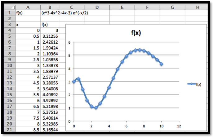
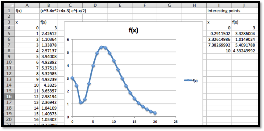
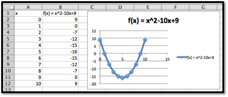
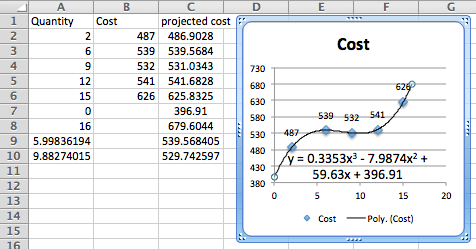
As always, we start by using simpler tools. In this case it is useful to have Excel sketch a graph and to use information we gathered in prior course. From the form of the function we know the graph is a parabola that points downwards.

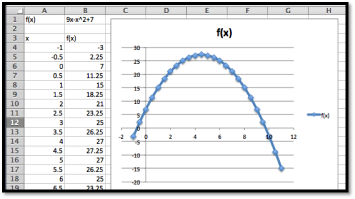
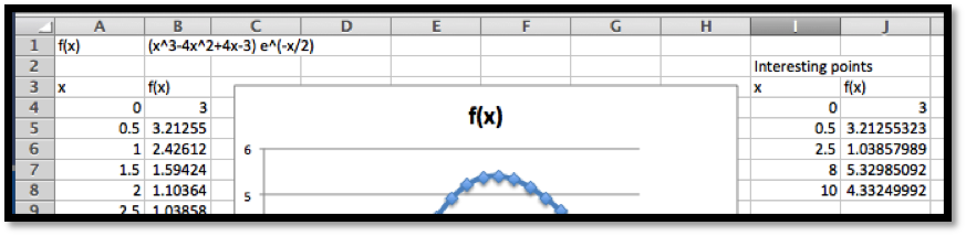
Looking at the chart and the picture we see that the vertex is close to $x=4.5\text{.}$ We also see that the x-intercepts are close to $x=-0.5$ and $x=9.5\text{.}$

Next, we want to make sure that Solver is installed. It should be on the Analysis section of the Data tab.

If you don’t find it there, you should go to the online help for Excel, and look for help on Solver. Under the topic “Define and solve a problem by using Solver”, select first “Define and solve a problem”, then “If you don’t see Solver under Analysis on the Data tab”.

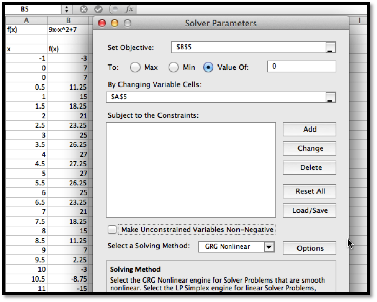
We first want to use Solver to find a root. Using the same approach we used with Goal Seek, we would like cell B5 to be set equal to 0 by changing the value of cell A5. (As we have set up the problem, we could use solver starting with any of the cells that give a value for $f(x)\text{.}$ I chose the one that has $f(x)$ closest to the desired result.)

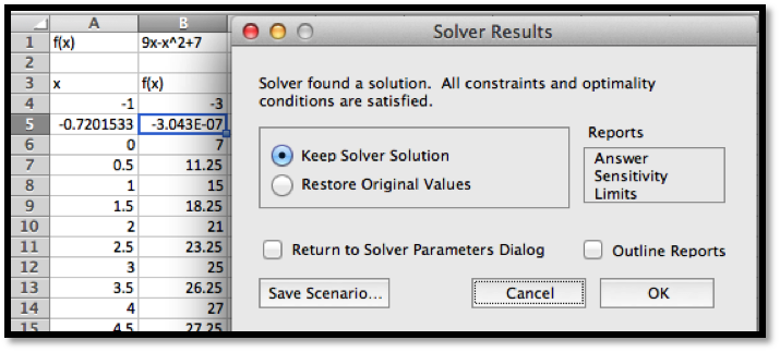
Solver finds a solution with $x=-0.72015\text{.}$ We are given a dialog box that asks if we want to keep the solver solution or restore our original value.

As with Goal Seek, if we use Solver again, starting with $x$ closer to 9, we will find a solution $x=9.72015\text{.}$

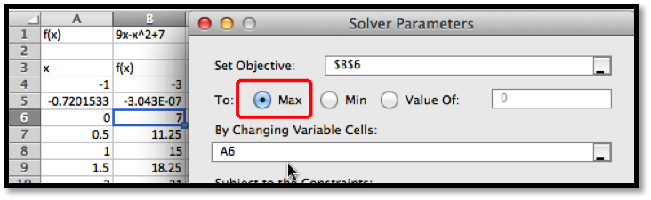
We introduce Solver because it can do things would be more difficult with Goal Seek. From the graph, and our knowledge or parabolas, we know the graph has a single maximum. To find the maximum with Goal Seek, we need to realize that the maximum occurs when the derivative is 0, define the numerical derivative, then set the derivative equal to 0. With Solver, we simply ask it to find the maximum. It finds the vertex at $x=4.5\text{.}$

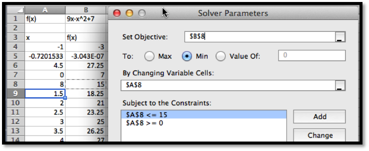
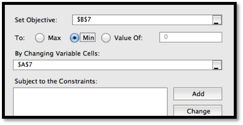
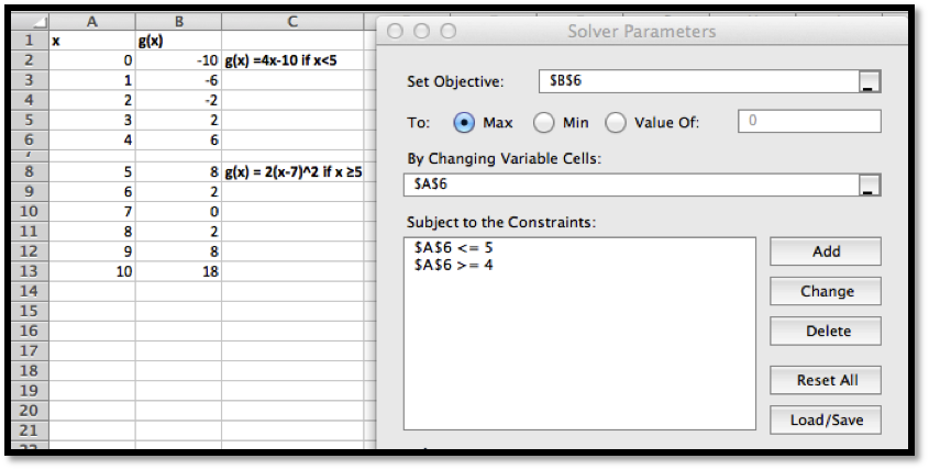
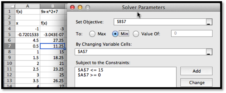
We also would like to be able to find a minimum. From the picture, we know that a downward pointing parabola has no absolute minimum. However, in business, we are typically concerned with functions defined on a finite domain. For this problem, consider only the interval $0\le x\le 15\text{.}$ We want the minimum to appear in cell B7, so we want to constrain cell A7. If we start Solver, then hit the add button, we get a dialog box to enter the first constraint, that A7$\ge 0\text{.}$

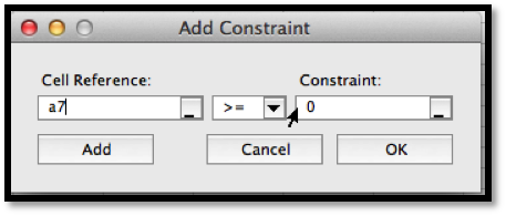
In a similar manner, we add the constraint that $A7\ge 15$ and ask solver for a minimum.

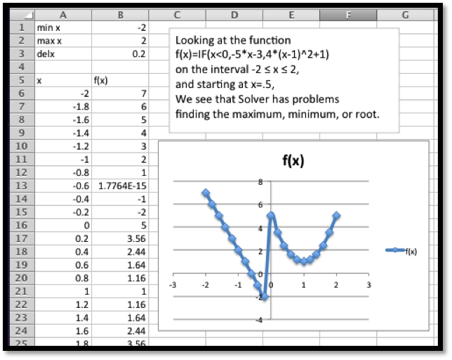
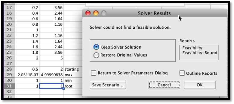
Since we started the search for the minimum at $x=0.5\text{,}$ Solver finds the minimum at $x=0\text{.}$ This is a “local minimum”. Any $x$ value in the interval that is close by gives a higher value for the function.

We would also like to find the minimum at the other end of the interval. To do that it is useful to know a bit of the mathematics behind what solver is doing. Solver uses derivatives from the starting point to decide on the direction it should look and how far it should go to find the next guess for its answer. This is a modification of a technique called Newton’s method. In terms of our picture, depending on whether we tell it to find a maximum, minimum, or specified value, Solver tries to slide up or down the graph until it finds a good candidate, which it gives us as a solution. It is actually looking for the first local maximum or minimum it gets to. It does not look for other candidates. So if we started at $x=0.5\text{,}$ it will slide to the left to find an answer. To find the minimum at the other end of the interval, we need a starting point where the graph is already sloping down to the right. Starting at $x=8$ should work. We set up Solver.

Solver finds that the curve had a minimum at $x=15$ with $f(x)=-83\text{.}$

To recap, using Solver on the interval $0\le x\le 15\text{,}$ we found has a root at $x=9.72015\text{,}$ a maximum at $x=4.5\text{,}$ and local minimums at $x=0$ and $x=15\text{.}$ We also found the values of $f(x)$ at all of those points.

It is worth pointing out that the default setting has "Make unconstrained variables non-negative. You generally want to turn that option off.

However, this example was chosen because we could get the same results with work by simply using the properties of parabolas. Thus, we now want to ask the same questions about a problem we cannot solve algebraically.

Example 3.5.8. A deceptive graph.

Figure 3.5.9. Video presentation of this example

Use solver to gather information, on the interval $0\le x\le 15\text{,}$ on the graph of $f(x)=(x^3-4x^2+4x+3) e^{(-x/2)}\text{.}$

Solution.

As always, start by looking at a graph.

From the graph I expect the function has no roots on the interval. It has local minimums near 0, 2.5, and 10. It has local maximums near 0.5, and 8. I will need to add constraints to find the local minimums at the boundaries. To make my worksheet easy to read I add two extra columns for the x and y values of interesting point, and fill in guesses.

After I use Solver, I find the local minimums occur at 0, 2.326, and 10, and the local maximums occur at 0.29115 and 7.3827. The maximum value for the function in the interval is 5.409 and the minimum is 1.0149. We verify that the endpoints, $x=0$ and $x=10\text{,}$ are both local minimums.

This function can be used to illustrate a limitation of our method. If we had graphed the functions at intervals at intervals of size 1 rather than 0.5, we get a different picture.

In that case, we miss the local maximum at 0.29 and confuse the left endpoint as a local maximum. Since Solver does not use the picture, it will not be misled by it. This example points out that while the graph is useful for guidance, we need to verify that we have not been misled by not graphing with enough resolution.

Warning: In Example 3.5.8 we saw that relying on the graph could deceive us. The flip side is an example where relying on Solver can deceive us. We mentioned earlier that Solver uses a variant of Newton’s method to find values. In rough terms, it repeatedly finds the linear approximation and slides up or down that line to the desired answer. If we start close to the answer, this is a very effective method of finding a numerical solution. However, it is easy to construct problems where this leads to a blind alley or to the wrong answer. In particular, the method has great difficulty with problems where the function is not differentiable or where it has several bends. Consider the following example.

Example 3.5.10. Deceiving Solver.

Figure 3.5.11. Video presentation of this example

Use solver to gather information, on the interval $-2\le x\le 2\text{,}$ on the graph of

\begin{equation*} f(x)=\begin{cases} -5x-3\amp x\lt 0\\ 4(x-1)^2 \amp x \gt 0\\ \end{cases}\text{.} \end{equation*}

Solution.

As always, start by looking at a graph. We use the IF function to produce cases.

It is pretty easy to see that the function reaches a maximum of 7 at $x=-2\text{,}$ and has a root at $x=-0.6\text{.}$ On this interval the function does not have a minimum, but it gets close to -3 when $x$ approaches 0 from the negative side. If we start at $x=0.5$ and try sliding up or down the curve, we are going in the wrong direction to find the root or minimum. To find the maximum we also need to go down before we can go up to the maximum.

When we look at solver, we get the wrong but expected results. The function not only fails to have a tangent line at $x=0\text{,}$ it has a jump there. Solver finds the nearest local maximum and minimum. For the root, it tells us it can’t find a feasible solution.

The lesson to learn is that solver will help us find our candidate points, but we still need to understand the functions behavior well enough to give a good starting point.

A preview of things to come — Extrema of functions of two variables.

There is another feature of Solver that we will come back to later in the course. Goal Seek asked which cell should be changed to reach our desired goal. Solver allows us to specify a number of cells that we can change. This means it will work with functions of several variables. This will allow us to shed some light on one of the “black boxes” we used earlier in this course, the ability of Excel to find a trendline, or best fitting curve to a set of data.

Example 3.5.12. Use solver to find a best fitting line to a data set.

Figure 3.5.13. Video presentation of this example

Find a best fitting line to the following data.

x	1	2	3	4	5
y	35	46	78	84	114

Solution.

As we mentioned in Section 1.4, when we are asked to find a best fitting line, we are asked to create a predicting function $p(x)=A x+B\text{,}$ with $A$ and $B$ chosen to minimize the sum of the squares of the error between the actual values and the predicted values. We build a worksheet that finds the sum of squared errors. We start with our variables, A and B, set at 5, an arbitrary initial guess.

We ask Solver to minimize D11 by changing B2 and B3. For comparison we ask for the best fitting Trendline using the scatterplot.

We see that we get the same answers, subject to rounding rules.

The Trendline tool has the advantage of being easier to use in many cases. Finding the best fitting curve with solver has the advantage of showing what we mean by best fitting. It will also work with models that may not have been programmed into the Trendline tool.

Checkpoint 3.5.14. Reading check, Optimization.

This question checks your reading comprehension of the material is section 3.5, An Introduction to Solver, of Business Calculus with Excel. Based on your reading, select all statements that are correct. There may be more than one correct answer. The statements may appear in what seems to be a random order.

Solver can run into problems when it has to move across a bend in the curve to find a solution.
Solver is more versatile than Goal Seek.
Solver can be used on functions of 2 variables.
Solver uses a version of Newton’s method to find extrema.
Solver will only find a root if the function actually has one.
Solver can find the minimum of any function.
It is easiest to think of solver as a more powerful version of Goal Seek.
None of the above

Exercises Exercises: An Introduction to Solver

Exercise Group.

In Exercise 3.5.1–3.5.7 you are given a function and an interval it is defined over:

Make a chart of values and plot a graph of the function.
Find any roots for the function.
Find relative maxima and minima for the function. (Remember to include the endpoints.).
Find the absolute maximum and minimum of the function on the interval.

1.

$f(x)=x^2-10x+9\text{,}$ on the interval $0\le x\le 10\text{.}$

Solution.

We can read off the roots from the table $f(x)=0$ at $x = 1$ and at $x = 9$
Use Solver to find the minimum.

Solver indicates that the minimum value of the function is -16 and the minimum takes place at $x = 5\text{.}$

We have local maximums at the endpoints $(0, 9)$ and $(10,9)\text{.}$
Test the endpoints,$(0, 9)$ and $(10,9)\text{,}$ and compare to the minimum, $(5, 16)\text{.}$

The absolute minimum is -16 (at $x = 5$) and the absolute maximum is 9 (at $x = 1$ and 10)

2.

$g(x)=10x*(4/5)^x-1\text{,}$ on the interval $0\le x\le 10\text{.}$

3.

$h(x)=(3000+200x) (0.97)^x\text{,}$ on the interval $0\le x\le 100\text{.}$

Solution.

This function does not have any roots on the interval $0\le x \le 100\text{.}$
The graph indicates there is a maximum near $x = 20\text{.}$ Use Solver: There is a maximum at $x = 17.83\text{.}$ The maximum value is 3814.53.

We have local minimums at the endpoints $(0, 3000)$ and $(100, 1093.71)\text{.}$
Compare the local extrema to the endpoints. We need to consider three points, $(100, 1093.71)\text{,}$ $(17.83, 3814.53)\text{,}$ and $(100, 1093.71)\text{.}$

The global maximum is 3814.53 (at $x = 17.83$).

The global minimum of 1093.71 (at $x = 100$).

4.

The revenue function, $\revenue(q)=(500-3q)(q)\text{,}$ on the interval $0\le q\le 200\text{.}$

5.

The profit function, $\profit(q)=(500-3q)(q)-(12q+600)\text{,}$ on the interval $0\le q\le 200\text{.}$

Solution.

There are 2 roots: one near $q = 0\text{,}$ and the other near $q = 160\text{.}$ Using Solver we find the roots are at $q = 1.24$ and $q = 161.43\text{.}$
The local maximum looks to be near $q = 80\text{.}$ Using solver we get a local maximum of $19,245.33 at $q = 81.33\text{.}$

We have local minimums at the endpoints $(0, -600)$ and $(200, -23000.)\text{.}$
Compare the local extrema to the endpoints. We need to consider three points, $(0, -600)\text{,}$ $(81.33, 19245.33)\text{,}$ and $(200, -23000)\text{.}$

The global maximum is 19245.33 (at $x = 81.33$).

The global minimum of -23000 (at $x = 200$).

6.

The profit function obtained as the best fitting quadratic curve for the following data.

Quantity	157	513	702	842	995
Profit	143,814	314,801	322,223	279,988	189,263

on the interval $0\le \quantity\le 1200\text{.}$

7.

The cost function obtained as the best fitting cubic curve for the following data.

Quantity	2	6	9	12	15
Cost	487	539	532	541	626

on the interval $0\le \quantity\le 16\text{.}$

Solution.

First we need to use Trendlines to find the equation of the function. Use polynomial of degree 3 to find the function

\begin{equation*} \cost(x)= 0.3353x^3 - 7.9874x^2 + 59.63x + 396.91\text{.} \end{equation*}

There are no roots on the interval $[0,16]\text{.}$
There is a local maximum between 4 and 8, and a local minimum between 8 and 12. Using Solver We find the local maximum at $(6.00, 539.57)$ and a local minimum at $(9.88, 529.74)\text{.}$ We also have a local minimum at the endpoint $(0, 396.91)$ and a local maximum at the other endpoint $(16, 679.604)\text{.}$
Compare the local extrema to the endpoints. We need to consider four points, $(0, \$396.91)\text{,}$ $(6.00, \$539.57)\text{,}$ $(9.88, \$529.74)\text{,}$ and $(16, \$584.30)\text{.}$

The global maximum is $396.91 (at $x = 0$)

The global minimum of $679.604 (at $x = 16$)

Exercise Group.

In Exercise 3.5.8–3.5.10 you are given a function that and an interval it is defined over.

Make a chart of values and plot a graph of the function.
Visually identify approximate local maxima and minima.
Find a reasonable range of starting points from which Solver will find each local maximum or minimum.

8.

$f(x)=-0.25x^4+5.3x^3-36x^2+90x-15\text{,}$ on the interval $0\le x\le 15\text{.}$

9.

\begin{equation*} g(x)=\begin{cases} 4x-10& x\lt 5\\ 2(x-7)^2&x \gt 5\\ \end{cases} \end{equation*}

on the interval $0\le x\le 10\text{.}$

Solution.

Inserting an empty row will allow us to see the break in the graph where we switch from the linear part to the quadratic part of the function. The functions have been included for clarity.
The local maximum looks to be at approximately $x = 5$ and the local minimum appears to be near $x = 7\text{.}$
The local minimum is the most straight forward: start at $x = 7$ and let Solver find the minimum. Solver indicates that the minimum value is 0 and the minimum occurs at $x = 7\text{.}$
For the local maximum we can have two things happen:
- The maximum is on the linear part of the equation.
- The maximum is on the quadratic part.
The two pieces do meet at $x = 5\text{,}$ but we cannot see just where the line ends up.

So start with $x = 4$ on Solver, find the maximum on the interval [4,5] and compare that to the value on the other branch of the graph.

Solver returns a value of 10 at $x = 5\text{.}$

Note that $g(x)$ is defined to be 8 exactly at $x = 5\text{,}$ because the output is determined by the $2(x-7)^2$ part.

Thus we do not have a local maximum here. The graph approaches 10 (gets infinitely close to it) as x approaches 5 from the left, but switches to 8 at he last minute.

10.

\begin{equation*} h(x)=\begin{cases} -4*(x-2)^2& x \lt 6\\ 2(x-7)^2-10&x \gt 6\\ \end{cases} \end{equation*}

on the interval $0\le x\le 10\text{.}$

You have attempted of activities on this page.

Prev Top Next