Definition of Best Fitting Curve.
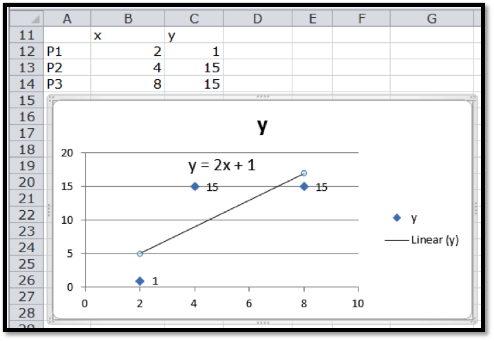
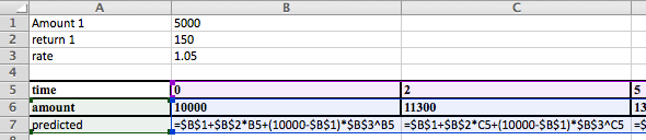
Before we can find the curve that is best fitting to a set of data, we need to understand how “best fitting” is defined. We start with the simplest nontrivial example. We consider a data set of 3 points, \({(1,0),(3,5),(6,5)}\) and a line that we will use to predict the y-value given the x-value, \(\predicted(x)=x/2 +1\text{.}\) We want to determine how well the line matches that data. For each point, \((x_i,y_i)\text{,}\) in the set we start by finding the corresponding point, \((x_i,\predicted(x_i ))\text{,}\) on the line.
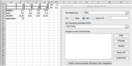
This gives us a set of predicted points, \({(1,1.5),(3,2.5),(6,4)}\text{.}\)
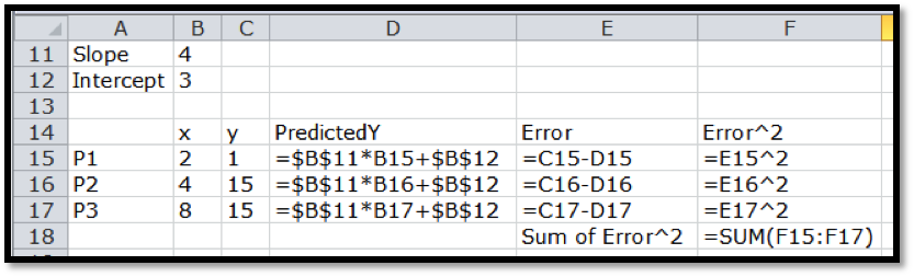
For each point we now compute the difference between the actual y-values and the predicted y-values. Our errors are the lengths of the brown segments in the picture, in this case \({3/2,3/2,1}\text{.}\) Finally we add the squares of the errors, \(9/4+9/4+1=11/2\text{.}\)
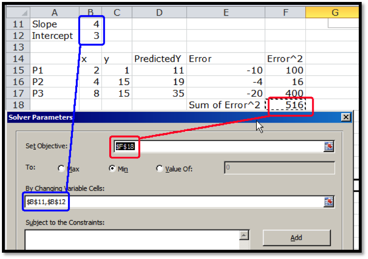
The best fitting line is defined to be the line that that minimizes the sum of the squares of the error. If we are trying to fit the data with a different model, we want to choose the equation from that model that minimizes the sum of the squares of the error.