10.4. Implementing the Sand Pile
To implement the sand pile model, We define a class called SandPile that inherits from Cell2D, which is defined in Cell2D.py in the repository for this book.
class SandPile(Cell2D):

    def __init__(self, n, m, level=9):
        self.array = np.ones((n, m)) * level
All values in the array are initialized to level, which is generally greater than the toppling threshold, K.
Here’s the step method that finds all cells above K and topples them:
kernel = np.array([[0, 1, 0],
                   [1,-4, 1],
                   [0, 1, 0]])

def step(self, K=3):
    toppling = self.array > K
    num_toppled = np.sum(toppling)
    c = correlate2d(toppling, self.kernel, mode='same')
    self.array += c
    return num_toppled
To show how step works, we will start with a small pile that has two cells ready to topple:
pile = SandPile(n=3, m=5, level=0)
pile.array[1, 1] = 4
pile.array[1, 3] = 4
Initially, pile.array looks like this:
[[0 0 0 0 0]
 [0 4 0 4 0]
 [0 0 0 0 0]]
Now we can select the cells that are above the toppling threshold:
toppling = pile.array > K
The result is a boolean array, but we can use it as if it were an array of integers like this:
[[0 0 0 0 0]
 [0 1 0 1 0]
 [0 0 0 0 0]]
If we correlate this array with the kernel, it makes copies of the kernel at each location where toppling is 1.
c = correlate2d(toppling, kernel, mode='same')
And here’s the result:
[[ 0  1  0  1  0]
 [ 1 -4  2 -4  1]
 [ 0  1  0  1  0]]
Notice that where the copies of the kernel overlap, they add up.
This array contains the change for each cell, which we use to update the original array:
pile.array += c
And here’s the result:
[[0 1 0 1 0]
 [1 0 2 0 1]
 [0 1 0 1 0]]
So that’s how step works.
With mode='same', correlate2d considers the boundary of the array to be fixed at zero, so any grains of sand that go over the edge disappear.
SandPile also provides run, which calls step until no more cells topple:
def run(self):
    total = 0
    for i in itertools.count(1):
        num_toppled = self.step()
        total += num_toppled
        if num_toppled == 0:
            return i, total
The return value is a tuple that contains the number of time steps and the total number of cells that toppled.
If you are not familiar with itertools.count, it is an infinite generator that counts up from the given initial value, so the for loop runs until step returns 0.
Finally, the drop method chooses a random cell and adds a grain of sand:
def drop(self):
   a = self.array
   n, m = a.shape
   index = np.random.randint(n), np.random.randint(m)
   a[index] += 1
Let’s look at a bigger example, with n=20:
pile = SandPile(n=20, level=10)
pile.run()

Gif of a sand pile running for 100 steps.

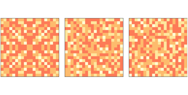
Figure 10.1: Sand pile model initial state (left), after 200 steps (middle), and 400 steps (right).
With an initial level of 10, this sand pile takes 332 time steps to reach equilibrium, with a total of 53,336 topplings. Figure 10.1 (left) shows the configuration after this initial run. Notice that it has the repeating elements that are characteristic of fractals. We’ll come back to that soon.
Figure 10.1 (middle) shows the configuration of the sand pile after dropping 200 grains onto random cells, each time running until the pile reaches equilibrium. The symmetry of the initial configuration has been broken; the configuration looks random.
Finally Figure 10.1 (right) shows the configuration after 400 drops. It looks similar to the configuration after 200 drops. In fact, the pile is now in a steady state where its statistical properties don’t change over time. We will learn about some of those statistical properties in the next section.