Grouping Data
Filtering data allows you to subset data to a set of rows based on some conditions. This allows for analysis on that subset of data. Finding summary statistics for a specific group of observations is called grouping. For example, if you have income data for the entire USA but want to find the mean income just for California, you would group the data by state.
Grouping can be done in Sheets using one of three “conditional summary” functions.
Grouping Functions in Sheets
The COUNTIF function counts the number of cells that satisfy a condition.
The syntax looks like =COUNTIF(cell range to be filtered, filter
condition).
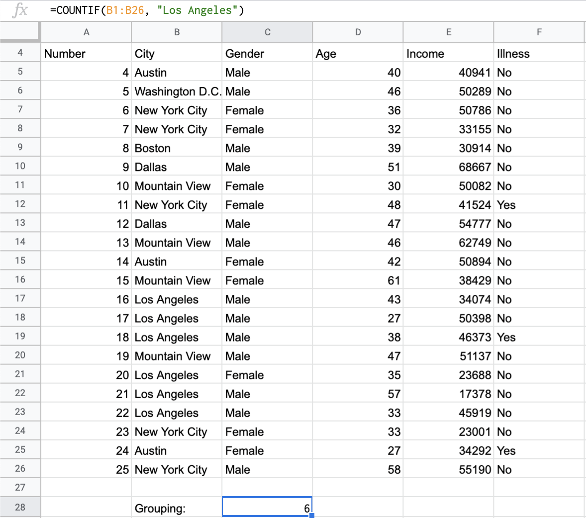
Earlier in the introduction you saw an example of the COUNTIF function
used on a table of standard information about people. That example utilizes
the formula =COUNTIF(B1:B26, “=Los Angeles”). This counts the number of
cells in the range B1:B26 that match the word “Los Angeles”. The cell range
to be filtered is B1:B26, and the filter condition is
“=Los Angeles”.
The SUMIF function sums the values of cells that satisfy a condition. The
syntax looks like =SUMIF(cell range to be filtered, filter condition, cell
range to be summed).
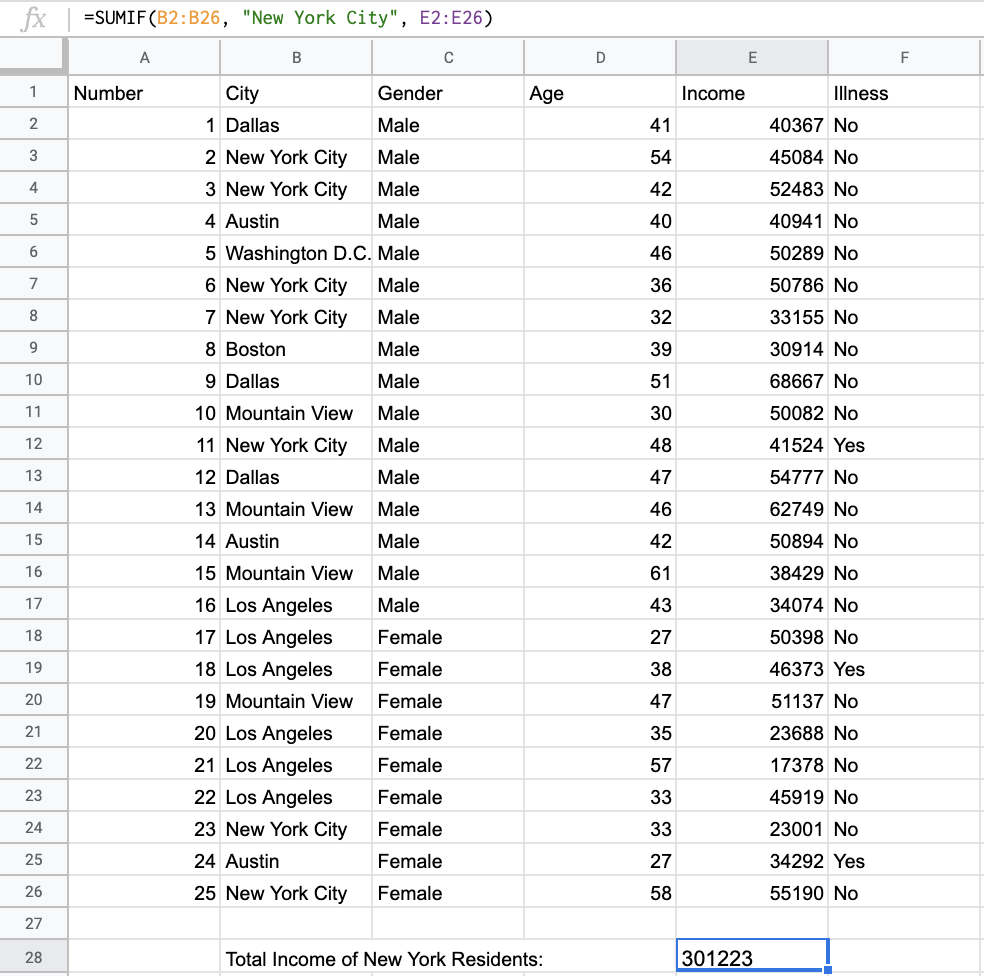
Given the same table of standard information about people, you can find the
total income of those from New York City. Consider the formula
=SUMIF(B2:B26, "=New York City", E2:E26). This sums the values in the
cells E2:E26, but only using rows for which the cell in that row in
column B matches the word “New York City”. The cell range to be filtered
is B2:B26, the filter condition is “=New York City”, and the
cell range to be summed is E2:E26.
Pictured is a screenshot of part of the dataset in Sheets with the grouping
function SUMIF.
The AVERAGEIF function finds the mean of cells that satisfy a condition.
The syntax looks like =AVERAGEIF(cell range to be filtered, filter
condition, cell range to be averaged).
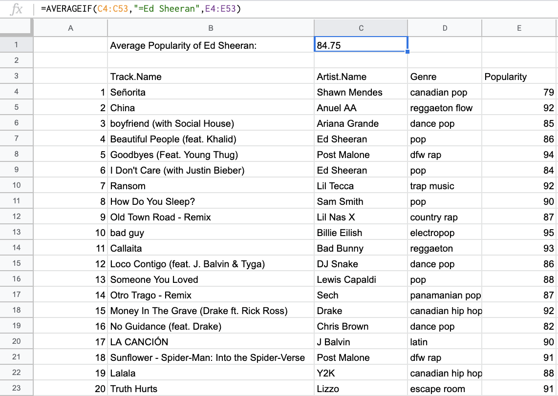
Given a table of the top 50 songs on Spotify in 2019, you can calculate
the mean popularity of songs by a certain artist. For example, consider the
formula =AVERAGEIF(C4:C53, "=Ed Sheeran", E4:E53). This finds the mean
of cells in the range E4:E53, but only using rows for which the cell in
that row in column C matches the word “Ed Sheeran.” The cell range to be
filtered is C4:C53, the filter condition is “=Ed Sheeran”, and
the cell range to be averaged is E4:E53.
Note that for SUMIF and AVERAGEIF, if you want to sum or average the
rows in column B or C themselves, you can enter B2:B26 or C2:C53 as the
third argument or leave the third argument empty.
Example: Painters
Grouping functions are most useful when finding summary statistics for a specific group. Consider the painters dataset, one last time. Suppose you want to count the number of French painters in this dataset, and find the total number of paintings made by those painters. This can be done using filtering or using grouping.
Create a filter to limit the dataset to only French painters. (For this example, assume “French” means the only nationality is French.) Copy the filtered table to a new sheet.
Q-1: Use COUNT on the filtered table to find the number of French painters.
Q-2: Use SUM on the filtered table to find the number of paintings by French
painters.
Why was it necessary to copy-paste the filtered data to new rows? Cell ranges do not behave well in filtered tables. This is best illustrated via an example. Consider the filter applied above, to limit the painters dataset to French painters.
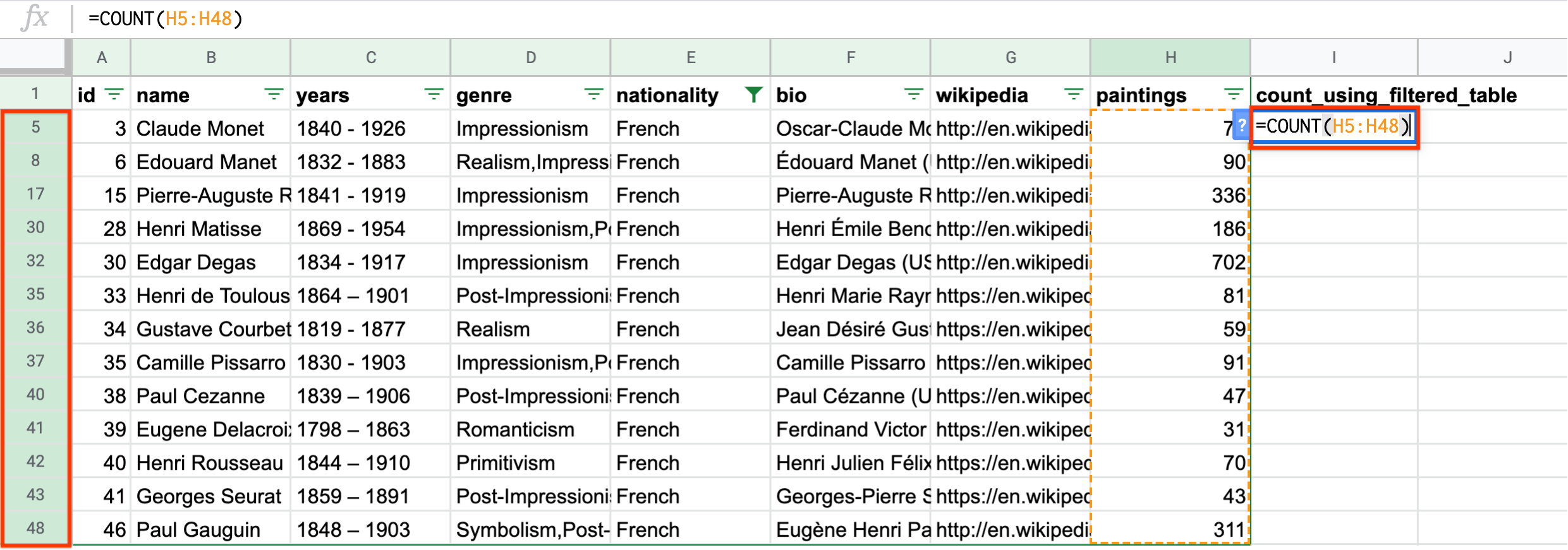
Notice that when trying to count the number of rows, selecting the cells selects
all cells between the first and the last, not just the filtered cells. Note that
the selected range is H5:H48`. While there are only 13 filtered rows, the
range selects all rows between 5 and 48. This returns a count of 44 French
artists, which is incorrect. The same is true for cell ranges when using ``SUM
and AVERAGE.
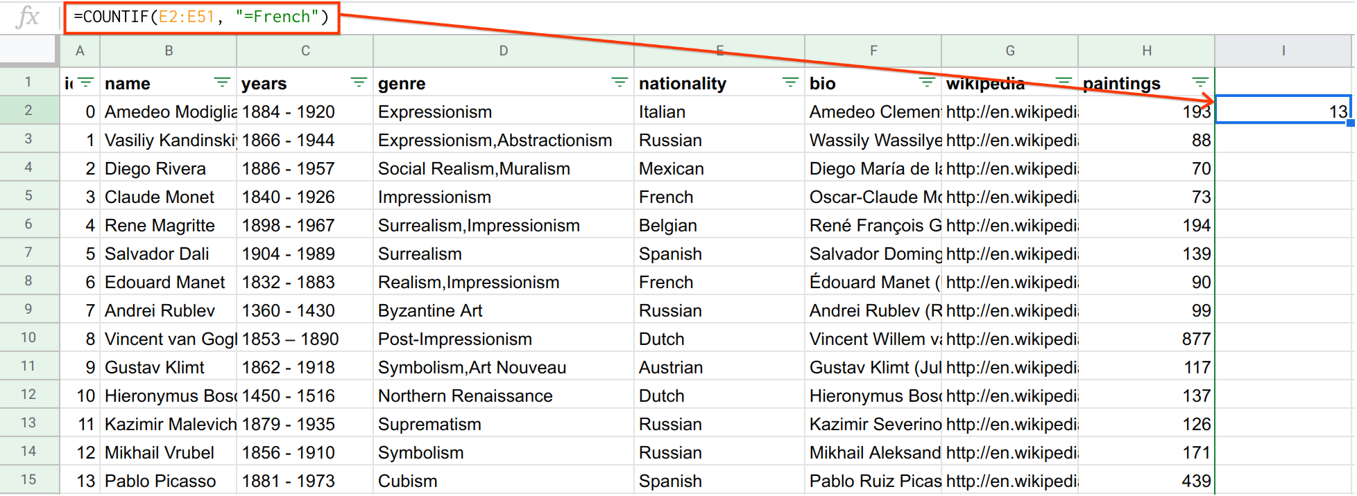
Instead of copy-pasting the filtered table to a new sheet and then using summary
functions, you can just use grouping functions. For example, to count the number
of French painters, you can use COUNTIF. The range to be counted is the
“nationality” column, and the column condition checks whether the value is
“French”.
Q-3: Use SUMIF to find the number of paintings by French painters.
Note that if you wanted to use the more general definition of “French” (any
painter who has French as one of their nationalities), you would need to use a
different filter condition. In general, the filter condition for checking if
“word” appears anywhere in the text looks like "*word*". This forum
discussion goes into more detail. This can apply to any grouping function.
Use grouping functions (COUNTIF, SUMIF, AVERAGEIF) when answering
the following questions.
Q-4: How many Italian (only nationality is Italian) painters are in the list?
Q-5: What is the mean number of paintings by Italian painters? (Round your answer to the nearest whole number.)
Impressionism
-
Correct
Romanticism
-
Incorrect
Q-6: Which genre produced more paintings: impressionism or romanticism? (You may simplify this by only looking at painters whose only genre is impressionism or romanticism.)
Q-7: How many painters were associated with multiple genres? (Hint: Look for painters whose “genre” field contains a comma.)
Example: Titanic
The Titanic was a passenger ship that sank on its journey from Southampton (England) to New York (USA) in 1912, killing over 1,500 people. This example uses passenger data from the tragedy. Each row records a passenger on the ship.
The purpose of this example is to find out whether some groups, for example, women and children who had priority access to life rafts in case of emergency, had a higher survival rate than others. For example, did women and children have a higher survival rate than men? This can be done very conveniently using grouping functions.
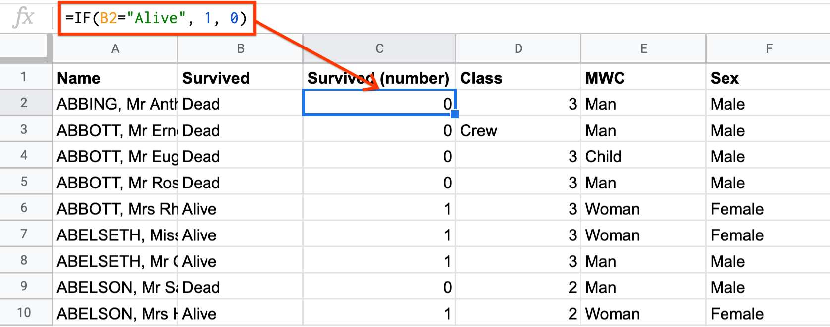
In its raw state, the survival of each passenger is encoded as “Dead” or “Alive” in column B. These words are hard to deal with numerically, so you should probably first transform these values to numbers. For example, the following formula maps “Dead” to 0 and “Alive” to 1. (The example is for cell B2, but it can be copy-pasted for the other rows.) You can insert a column on the left of column C and use this column for the formula.
=IF(B2=“Alive”, 1, 0)
Q-8: What is the survival rate on the Titanic? (Give your answers as a percentage, to two decimal places.) %
This survival rate you just calculated is the overall survival rate for all passengers. What if you want to know the survival rate just for men, or just for women, or just for children?
To calculate the survival rate just for men, you need to find the mean of column
C, but only if column E is equal to “Man”. This is a perfect use case for
AVERAGEIF.
=AVERAGEIF(E$2:E$2209, "=Man", C$2:C$2209)

Q-9: What is the survival rate for women? (Give your answers as a percentage, to two decimal places.) %
Q-10: What is the survival rate for children? (Give your answers as a percentage, to two decimal places.) %
Q-11: Compare the survival rate across the classes: Crew, Class 3, Class 2, Class 1. Is this in line with what you expected?