5.12. Dynamic Programming
Dynamic programming is a technique of breaking the main problem into smaller subproblems and then using those subproblems to construct the answer to the main problem.
Many programs in computer science are written to optimize some value; for example, find the shortest path between two points, find the line that best fits a set of points, or find the smallest set of objects that satisfies some criteria. There are many strategies that computer scientists use to solve these problems. One of the goals of this book is to expose you to several different problem solving strategies. Dynamic programming is one strategy for these types of optimization problems.
A classic example of an optimization problem involves making change using the fewest coins. Suppose you are a programmer for a vending machine manufacturer. Your company wants to streamline effort by giving out the fewest possible coins in change for each transaction. Suppose a customer puts in a dollar bill and purchases an item for 37 cents. What is the smallest number of coins you can use to make change? The answer is six coins: two quarters, one dime, and three pennies. How did we arrive at the answer of six coins? We start with the largest coin in our arsenal (a quarter) and use as many of those as possible, then we go to the next lowest coin value and use as many of those as possible. This first approach is called a greedy method because we try to solve as big a piece of the problem as possible right away.
The greedy method works fine when we are using U.S. coins, but suppose that your company decides to deploy its vending machines in Lower Elbonia where, in addition to the usual 1, 5, 10, and 25 cent coins they also have a 21 cent coin. In this instance our greedy method fails to find the optimal solution for 63 cents in change. With the addition of the 21 cent coin the greedy method would still find the solution to be six coins. However, the optimal answer is three 21 cent pieces.
Let’s look at a method where we could be sure that we would find the optimal answer to the problem. Since this section is about recursion, you may have guessed that we will use a recursive solution. Let’s start with identifying the base case. If we are trying to make change for the same amount as the value of one of our coins, the answer is easy, one coin.
If the amount does not match we have several options. What we want is the minimum of a penny plus the number of coins needed to make change for the original amount minus a penny, or a nickel plus the number of coins needed to make change for the original amount minus five cents, or a dime plus the number of coins needed to make change for the original amount minus ten cents, and so on. So the number of coins needed to make change for the original amount can be computed according to the following:
The algorithm for doing what we have just described is shown in Listing 7. In line 7 we are checking our base case; that is, we are trying to make change in the exact amount of one of our coins. If we do not have a coin equal to the amount of change, we make recursive calls for each different coin value less than the amount of change we are trying to make. Line 6 shows how we filter the list of coins to those less than the current value of change using a list comprehension. The recursive call also reduces the total amount of change we need to make by the value of the coin selected. The recursive call is made in line 14. Notice that on that same line we add 1 to our number of coins to account for the fact that we are using a coin. Just adding 1 is the same as if we had made a recursive call asking where we satisfy the base case condition immediately.
Listing 7
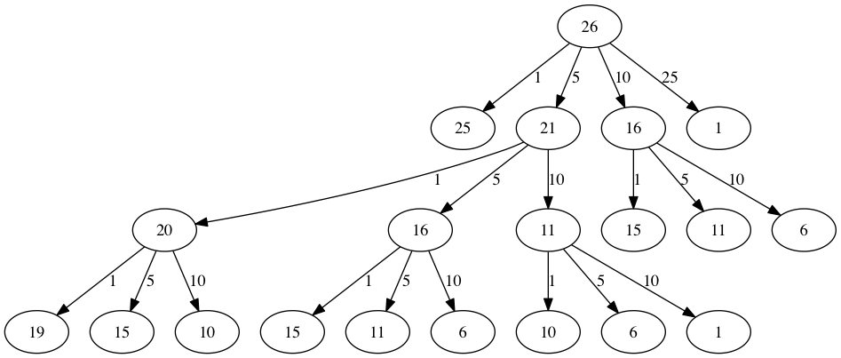
The trouble with the algorithm in Listing 7 is that it is extremely inefficient. In fact, it takes 67,716,925 recursive calls to find the optimal solution to the 4 coins, 63 cents problem! To understand the fatal flaw in our approach look at Figure 5, which illustrates a small fraction of the 377 function calls needed to find the optimal set of coins to make change for 26 cents.
Each node in the graph corresponds to a call to recMC. The label on
the node indicates the amount of change for which we are computing the
number of coins. The label on the arrow indicates the coin that we just
used. By following the graph we can see the combination of coins that
got us to any point in the graph. The main problem is that we are
re-doing too many calculations. For example, the graph shows that the
algorithm would recalculate the optimal number of coins to make change
for 15 cents at least three times. Each of these computations to find
the optimal number of coins for 15 cents itself takes 52 function calls.
Clearly we are wasting a lot of time and effort recalculating old
results.

Figure 3: Call Tree for Listing 7
The key to cutting down on the amount of work we do is to remember some of the past results so we can avoid recomputing results we already know. A simple solution is to store the results for the minimum number of coins in a table when we find them. Then before we compute a new minimum, we first check the table to see if a result is already known. If there is already a result in the table, we use the value from the table rather than recomputing. This technique is called memoization and is a very useful method for speeding up frequent yet hardware-demanding function calls. ActiveCode 1 shows a modified algorithm to incorporate our table lookup scheme.
Notice that in line 15 we have added a test to see if our table contains the minimum number of coins for a certain amount of change. If it does not, we compute the minimum recursively and store the computed minimum in the table. Using this modified algorithm reduces the number of recursive calls we need to make for the four coin, 63 cent problem to 221 calls!
Although the algorithm in AcitveCode 1 is correct, it looks and
feels like a bit of a hack. Also, if we look at the knownResults lists
we can see that there are some holes in the table. In fact the term for
what we have done is not dynamic programming but rather we have improved
the performance of our program by using a technique known as
“memoization,” or more commonly called “caching.” Memoization uses what is sometimes
called an opportunistic top-down approach. When you need the result of a computation,
you check to see if you have already computed it, otherwise you do the new
calculation and store the result.
A truly dynamic programming algorithm will take a more systematic bottom-up approach to the problem. Memoization and dynamic programming are both code optimization techniques that avoid recalculating duplicate work. Our dynamic programming solution is going to start with making change for one cent and systematically work its way up to the amount of change we require. This guarantees us that at each step of the algorithm we already know the minimum number of coins needed to make change for any smaller amount.
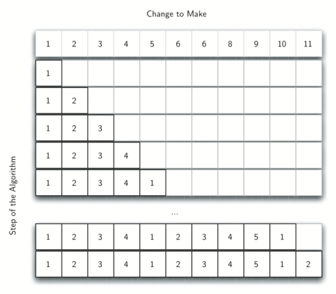
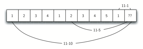
This is often called dynamic programming with tabulation. Let’s look at how we would fill in a table of minimum coins to use in making change for 11 cents. Figure 4 illustrates the process. We start with one cent. The only solution possible is one coin (a penny). The next row shows the minimum for one cent and two cents. Again, the only solution is two pennies. The fifth row is where things get interesting. Now we have two options to consider, five pennies or one nickel. How do we decide which is best? We consult the table and see that the number of coins needed to make change for four cents is four, plus one more penny to make five, equals five coins. Or we can look at zero cents plus one more nickel to make five cents equals 1 coin. Since the minimum of one and five is one we store 1 in the table. Fast forward again to the end of the table and consider 11 cents. Figure 5 shows the three options that we have to consider:
A penny plus the minimum number of coins to make change for \(11-1 = 10\) cents (1)
A nickel plus the minimum number of coins to make change for \(11 - 5 = 6\) cents (2)
A dime plus the minimum number of coins to make change for \(11 - 10 = 1\) cent (1)
Either option 1 or 3 will give us a total of two coins which is the minimum number of coins for 11 cents.

Figure 4: Minimum Number of Coins Needed to Make Change

Figure 5: Three Options to Consider for the Minimum Number of Coins for Eleven Cents
Listing 8 is a dynamic programming algorithm to solve our
change-making problem. dpMakeChange takes three parameters: a list
of valid coin values, the amount of change we want to make, and a list
of the minimum number of coins needed to make each value. When the
function is done minCoins will contain the solution for all values
from 0 to the value of change.
Listing 8
Note that dpMakeChange is not a recursive function, even though we
started with a recursive solution to this problem. It is important to
realize that just because you can write a recursive solution to a
problem does not mean it is the best or most efficient solution. The
bulk of the work in this function is done by the loop that starts on
line 4. In this loop we consider using all possible coins to
make change for the amount specified by cents. Like we did for the
11 cent example above, we remember the minimum value and store it in our
minCoins list.
Although our making change algorithm does a good job of figuring out the
minimum number of coins, it does not help us make change since we do not
keep track of the coins we use. We can easily extend dpMakeChange to
keep track of the coins used by simply remembering the last coin we add
for each entry in the minCoins table. If we know the last coin
added, we can simply subtract the value of the coin to find a previous
entry in the table that tells us the last coin we added to make that
amount. We can keep tracing back through the table until we get to the
beginning.
ActiveCode 2 shows the dpMakeChange algorithm
modified to keep track of the coins used, along with a function
printCoins that walks backward through the table to print out the
value of each coin used.
This shows the algorithm in
action solving the problem for our friends in Lower Elbonia. The first
two lines of main set the amount to be converted and create the list of coins used. The next two
lines create the lists we need to store the results. coinsUsed is a
list of the coins used to make change, and coinCount is the minimum
number of coins used to make change for the amount corresponding to the
position in the list.
Notice that the coins we print out come directly from the coinsUsed
array. For the first call we start at array position 63 and print 21.
Then we take \(63 - 21 = 42\) and look at the 42nd element of the
list. Once again we find a 21 stored there. Finally, element 21 of the
array also contains 21, giving us the three 21 cent pieces.
5.13. Summary
In this chapter we have looked at examples of several recursive algorithms. These algorithms were chosen to expose you to several different problems where recursion is an effective problem-solving technique. The key points to remember from this chapter are as follows:
All recursive algorithms must have a base case.
A recursive algorithm must change its state and make progress toward the base case.
A recursive algorithm must call itself (recursively).
Recursion can take the place of iteration in some cases.
Recursive algorithms often map very naturally to a formal expression of the problem you are trying to solve.
Recursion is not always the answer. Sometimes a recursive solution may be more computationally expensive than an alternative algorithm.
5.14. Self-check
- It must progress from the base case
- If it starts at the base case, then when would it stop?
- It must move towards the base case
- Correct. The base case is your endpoint.
- It must have a base case
- Correct. The base case is essential if you want a stopping point
- It must call itself
- Correct. If it doesn't call itself then it won't repeat
Q-9: What are the three laws of recursion for an algorithm? (choose all that are correct)
-
Q-10: Which implementation would be ideal for each problem.
Consider what would make you stop the process for each one.
- Counting the number of items in a list
- Iteration
- Going through an entire tree
- Recursion
- True
- Correct! Sometimes simple problems only need simple solutions, like a loop
- False
- Incorrect. Recursion is not always the ideal solution.
Q-11: Sometimes recursion can be more computationally expensive than an alternative, True or False?