
8.6. Graphs Revisited: Pattern Matching
Even with the growing interest in computer graphics, processing textual information is still an important area of study. Of particular interest here is the problem of finding patterns, often referred to as substrings, that exist in long strings of characters. The task is to perform some type of search that can identify at least the first occurrence of the pattern. We can also consider an extension of this problem to find all such occurrences.
Python includes a built-in substring method called find that returns
the location of the first occurrence of a pattern in a given string. For
example,
>>> "ccabababcab".find("ab")
2
>>> "ccabababcab".find("xyz")
-1
>>>
shows that the substring "ab" occurs for the first time starting at
index position 2 in the string "ccabababcab". find also returns
a -1 if the pattern does not occur.
8.6.1. Biological Strings
Some of the most exciting work in algorithm development is currently taking place in the domain of bioinformatics; in particular, finding ways to manage and process large quantities of biological data. Much of this data takes the form of coded genetic material stored in the chromosomes of individual organisms. Deoxyribonucleic acid, more commonly known as DNA, is a very simple organic molecule that provides the blueprint for protein synthesis.
DNA is basically a long sequence consisting of four chemical bases: adenine(A), thymine(T), guanine(G), and cytosine(C). These four symbols are often referred to as the genetic alphabet and we represent a piece of DNA as a string or sequence of these base symbols. For example, the DNA string ATCGTAGAGTCAGTAGAGACTADTGGTACGA might code a very small part of a DNA strand. It turns out that within these long strings, perhaps thousands and thousands of base symbols long, small pieces exist that provide extensive information as to the meaning of this genetic code. We can see then that having methods for searching out these pieces is a very important tool for the bioinformatics researcher.
Our problem then reduces to the following ideas. Given a string of symbols from the underlying alphabet A, T, G, and C, develop an algorithm that will allow us to locate a particular pattern within that string. We will often refer to the DNA string as the text. If the pattern does not exist, we would like to know that as well. Further, since these strings are typically quite long, we need to be sure that the algorithm is efficient.
8.6.2. Simple Comparison
Our first approach is likely the solution that comes immediately to your mind for solving the DNA string pattern-matching problem. We will simply try all possibilities for matching the pattern to the text. Figure 1 shows how the algorithm will work. We will start out comparing the pattern from left to right with the text, starting at the first character in both. If there is a match, then we proceed to check the second character. Whenever a mismatch occurs, we simply slide the pattern one position to the right and start over.
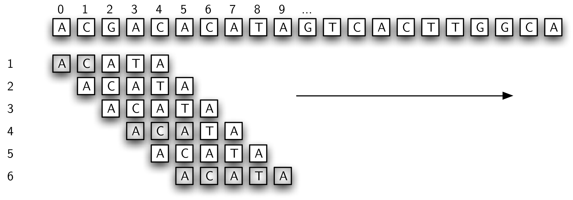
A Simple Pattern-Matching Algorithm
In this example, we have found a match on the sixth attempt, starting at
position 5. The shaded characters denote the partial matches that
occurred as we moved the pattern.
Listing [lst_simplematcher] shows the Python
implementation for this method. It takes the pattern and the text as
parameters. If there is a pattern match, it returns the position of the
starting text character. Otherwise, it returns -1 to signal that the
search failed.
def simple_matcher(pattern, text):
   i = j = 0

   while True:
      if text[i] == pattern[j]:
            j = j + 1
      else:
            j = 0
      i = i + 1

      if i == len(text):
            return -1
      if j == len(pattern):
            return i - j
The variables i and j serve as indices into the text and pattern
respectively. The loop repeats until either the text or the pattern
ends.
Line [lst_simplematcher:line_checkmatch] checks for a match between the current text character and the current pattern character. If the match occurs, pattern index is incremented. If the match fails, we reset the pattern back to its beginning (line [lst_simplematcher:line_patternreset]). In both cases we move to the next position in the text. At every iteration of the loop we check if there is more text to process (line [lst_simplematcher:line_textended]) and return -1 if not. Line [lst_simplematcher:line_patternended] checks to see if every character in the pattern has been processed. If so, a match has been found and we return its starting index.
If we assume that the length of the text is \(n\) characters and the length of the pattern is \(m\) characters, then it is easy to see that the complexity of this approach is \(O(nm)\). For each of the \(n\) characters we may have to compare against almost all \(m\) of the pattern characters. This is not so bad if the size of \(n\) and \(m\) are small. However, if we are considering thousands (or perhaps millions) of characters in our text in addition a large pattern, it will be necessary to look for a better approach.
8.6.3. Using Graphs: Finite State Automata
It is possible to create an \(O(n)\) pattern matcher if we are willing to do some preprocessing with the pattern. One approach is to build what is known as a deterministic finite automaton, or DFA, that represents the pattern as a graph. Each vertex of the DFA graph is a state, keeping track of the amount of the pattern that has been seen so far. Each edge of the graph represents a transition that takes place after processing a character from the text.
Figure 2 shows a DFA for the example pattern from the last section (ACATA). The first vertex (state 0) is known as the start state (or initial state) and denotes that we have not seen any matching pattern characters so far. Clearly, before processing the first text character, this is the situation.
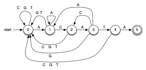
A Deterministic Finite Automaton
The DFA works in a very simple way. We keep track of our current state, setting it to 0 when we start. We read the next character from the text. Depending on the character, we follow the appropriate transition to the next state, which in turn becomes the new current state. By definition, each state has one and only one transition for each character in the alphabet. This means that for our DNA alphabet we know that each state has four possible transitions to a next state. Note that in the figure we have labeled some edges (transitions) with multiple alphabet symbols to denote more than one transition to the same state.
We continue to follow transitions until a termination event occurs. If we enter state 5, known as the final state (the two concentric circles denote the final state in the DFA graph), we can stop and report success. The DFA graph has discovered an occurrence of the pattern. You might note that there are no transitions out of the final state, meaning that we must stop at that point. The location of the pattern can be computed from the location of the current character and the size of the pattern. On the other hand, if we run out of text characters and the current state is somewhere else in the DFA, known as a nonfinal state, we know that the pattern did not occur.
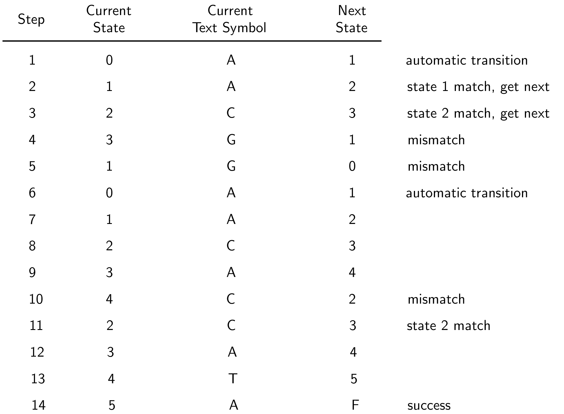
Figure 3 shows a step-by-step trace of the example DFA as it works through the text string ACGACACATA looking for the substring ACATA. The next state computed by the DFA always becomes the current state in the subsequent step. Since there is one and only one next state for every current state–current character combination, the processing through the DFA graph is easy to follow.

A Trace of the DFA Pattern Matcher
Since every character from the text is used once as input to the DFA graph, the complexity of this approach is \(O(n)\). However, we need to take into account the preprocessing step that builds the DFA. There are many well-known algorithms for producing a DFA graph from a pattern. Unfortunately, all of them are quite complex mostly due to the fact that each state (vertex) must have a transition (edge) accounting for each alphabet symbol. The question arises as to whether there might be a similar pattern matcher that employs a more streamlined set of edges.
8.6.4. Using Graphs: Knuth-Morris-Pratt
Recall the simple pattern matcher presented earlier. Every possible substring of the text was tested against the pattern. In many cases this proved to be a waste of time since the actual starting point for the match was farther down the text string. A possible solution to this inefficiency would be to slide the pattern more than one text character if a mismatch occurs. Figure 4 shows this strategy using the rule that we slide the pattern over to the point where the previous mismatch happened.
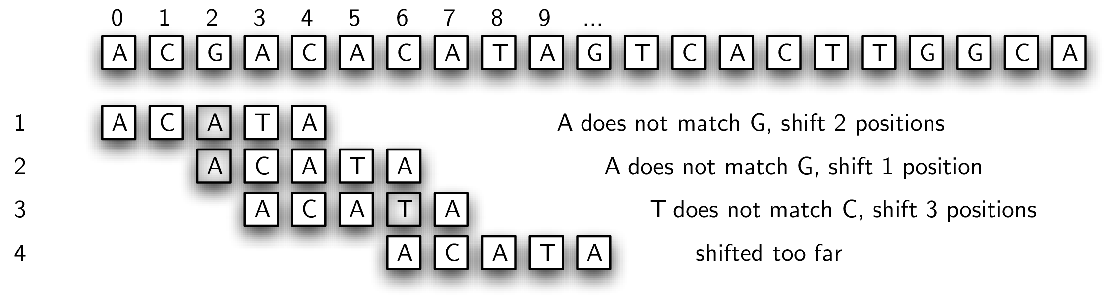
Simple Pattern Matcher with Longer Shifts
In step 1, we find that the first two positions match. Since the mismatch occurs in the third character (the shaded character), we slide the entire pattern over and begin our next match at that point. In step 2, we fail immediately so there is no choice but to slide over to the next position. Now, the first three positions match. However, there is a problem. When the mismatch occurs, our algorithm says to slide over to that point. Unfortunately, this is too far and we miss the actual starting point for the pattern in the text string (position 5).
The reason this solution failed is that we did not take advantage of information about the content of the pattern and the text that had been seen in a previously attempted match. Note that in step 3, the last two characters of the text string that occur at the time of the mismatch (positions 5 and 6) actually match the first two characters of the pattern. We say that a two-character prefix of the pattern matches a two-character suffix of the text string processed up to that point. This is valuable information. Had we been tracking the amount of overlap between prefixes and suffixes, we could have simply slid the pattern two characters, which would have put us in the right place to start step 4.
This observation leads to a pattern matcher known as Knuth-Morris-Pratt (or KMP), named for the computer scientists who first presented it. The idea is to build a graph representation that will provide information as to the amount of “slide” that will be necessary when a mismatch occurs. The KMP graph will again consist of states and transitions (vertices and edges). However, unlike the DFA graph from the previous section, there will be only two transitions leaving each state.
Figure 5 shows the complete KMP graph for the example pattern. There are two special states for a KMP graph, the initial state and the final state. The initial state, marked “get,” is responsible for reading the next character from the input text. The subsequent transition, marked with an asterisk, is always taken. Note that the start transition enters this initial state, which means that we initially get the first character from the text and transition immediately to the next state (state 1). The final state (state 6), this time labeled with an “F,” again means success and represents a termination point for the graph.
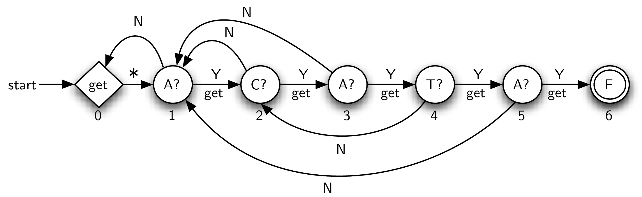
An Example KMP Graph
Each remaining vertex is responsible for checking a particular character of the pattern against the current text character. For example, the vertex labeled “C?” asks whether the current text character is C. If so, then the edge labeled “Y” is used. This means “yes,” there was a match. In addition, the next character is read. In general, whenever a state is successful in matching the character it is responsible for, the next character is read from the text.
The remaining transitions, those labeled “N,” denote that a mismatch occurred. In this case, as was explained above, we need to know how many positions to slide the pattern. In essence, we want to keep the current text character and simply move back to a previous point in the pattern. To compute this, we use a simple algorithm that basically checks the pattern against itself, looking for overlap between a prefix and a suffix (see Listing [lst_mismatchedlinks]). If such an overlap is found, its length tells us how far back to place the mismatched link in the KMP graph. It is important to note that new text characters are not processed when a mismatched link is used.
def mismatched_links(pattern):
    aug_pattern = "0" + pattern
    links = {1: 0}
    for k in range(2, len(aug_pattern)):
        s = links[k - 1]
        while s >= 1:
            if aug_pattern[s] == aug_pattern[k - 1]:
                break
            else:
                s = links[s]
        links[k] = s + 1
    return links
Here is the example pattern as it is being processed by the
mismatched_links method:
>>> mismatched_links("ACATA")
{1: 0, 2: 1, 3: 1, 4: 2, 5: 1}
>>>
The value returned by the method is a dictionary containing key-value pairs where the key is the current vertex (state) and the value is its destination vertex for the mismatched link. It can be seen that each state, from 1 to 5 corresponding to each character in the pattern, has a transition back to a previous state in the KMP graph.
As we noted earlier, the mismatched links can be computed by sliding the
pattern past itself looking for the longest matching prefix and suffix.
The method begins by augmenting the pattern so that the indices on the
characters match the vertex labels in the KMP graph. Since the initial
state is state 0, we have used the “0” symbol as a placeholder. Now the
characters 1 to \(m\) in the augmented pattern correspond directly
with the states 1 to \(m\) in the graph.
Line [lst_mismatchedlinks:line_initdict] creates the first dictionary entry, which is always a transition from vertex 1 back to the initial state where a new character is automatically read from the text string. The iteration that follows simply checks larger and larger pieces of the pattern, looking for prefix and suffix overlap. If such an overlap occurs, the length of the overlap can be used to set the next link.
Figure 6 shows the KMP graph as it is being used to locate the example pattern in the text string ACGACACATA. Again, notice that the current character changes only when a match link has been used. In the case of a mismatch, as in steps 4 and 5, the current character remains the same. It is not until step 6, when we have transitioned all the way back to state 0, that we get the next character and return to state 1.
Steps 10 and 11 show the importance of the proper mismatched link. In step 10 the current character, C, does not match the symbol that state 4 needs to match. The result is a mismatched link. However, since we have seen a partial match at that point, the mismatched link reverts back to state 2 where there is a correct match. This eventually leads to a successful pattern match.
A Trace of the KMP Pattern Matcher
As with the DFA graph from the previous section, KMP pattern matching is \(O(n)\) since we process each character of the text string. However, the KMP graph is much easier to construct and requires much less storage as there are only two transitions from every vertex.