ORCCA Exploring Two-Variable Data and Rate of Change

Section 3.3 Exploring Two-Variable Data and Rate of Change

This section is about examining data that has been plotted on a Cartesian coordinate system, and then making observations. In some cases, we’ll be able to turn those observations into useful mathematical calculations.

Figure 3.3.1. Alternative Video Lesson

Subsection 3.3.1 Modeling data with two variables

Using mathematics, we can analyze data from the world around us. We can use what we discover to understand the world better and make predictions. Here’s an example with economic data from the US, plotted in a Cartesian plane.

For the years from 1990 to 2013, consider what percent of all income was held by the top 1% of wage earners. The table in Figure 2 gives the numbers, but any pattern there might not be apparent when looking at the data organized this way. Plotting the data in a Cartesian coordinates sytem can make an overall pattern or trend become visible.

year	%	year	%
1990	14	2002	17
1991	13	2003	18
1992	15	2004	20
1993	14	2005	22
1994	14	2006	23
1995	15	2007	24
1996	17	2008	21
1997	18	2009	18
1998	19	2010	20
1999	20	2011	20
2000	22	2012	22
2001	18	2013	20

$a scatter plot about share of all income held by the top 1% in the US$

Figure 3.3.2. Share of all income held by the top 1% of wage earners

If this trend continues, what percentage of all income will the top 1 % have in the year 2030? If we model data in the chart with the trend line, we can estimate the value to be 28.6 %. This is one way math is used in real life.

Does that trend line have an equation like those we looked at in Section 2? Is it even correct to look at this data set and decide that a straight line is a good model?

Subsection 3.3.2 Patterns in Tables

Example 3.3.3.

Find a pattern in each table. What is the missing entry in each table? Can you describe each pattern in words and/or mathematics?

black	white
big	small
short	tall
few

USA	Washington
UK	London
France	Paris
Mexico

1	2
2	4
3	6
5

Figure 3.3.4. Patterns in 3 tables

Explanation.

black	white
big	small
short	tall
few	many

USA	Washington
UK	London
France	Paris
Mexico	Mexico City

1	2
2	4
3	6
5	10

Figure 3.3.5. Patterns in 3 tables

First table: Each word on the right has the opposite meaning of the word to its left.
Second table: Each city on the right is the capital of the country to its left.
Third table: Each number on the right is double the number to its left.

We can view each table as assigning each input in the left column a corresponding output in the right column. In the first table, for example, when the input “big” is on the left, the output “small” is on the right. The first table’s function is to output a word with the opposite meaning of each input word. (This is not a numerical example.)

The third table is numerical. And its function is to take a number as input, and give twice that number as its output. Mathematically, we can describe the pattern as “$y=2x\text{,}$” where $x$ represents the input, and $y$ represents the output. Labeling the table mathematically, we have Figure 6.

$x$ (input)	$y$ (output)
$1$	$2$
$2$	$4$
$3$	$6$
$5$	$10$
$10$	$20$
Pattern: $y=2x$

Figure 3.3.6. Table with a mathematical pattern

The equation $y=2x$ summarizes the pattern in the table. For each of the following tables, find an equation that describes the pattern you see. Numerical pattern recognition may or may not come naturally for you. Either way, pattern recognition is an important mathematical skill that anyone can develop. Solutions for these exercises provide some ideas for recognizing patterns.

Checkpoint 3.3.7.

Write an equation in the form $y=\ldots$ suggested by the pattern in the table.

$x$	$y$
$0$	${10}$
$1$	${11}$
$2$	${12}$
$3$	${13}$

Explanation.

One approach to pattern recognition is to look for a relationship in each row. Here, the $y$-value in each row is always $10$ more than the $x$-value. So the pattern is described by the equation ${y = x+10}\text{.}$

Checkpoint 3.3.8.

Write an equation in the form $y=\ldots$ suggested by the pattern in the table.

$x$	$y$
$0$	${-1}$
$1$	${2}$
$2$	${5}$
$3$	${8}$

Explanation.

The relationship between $x$ and $y$ in each row is not as clear here. Another popular approach for finding patterns: in each column, consider how the values change from one row to the next. From row to row, the $x$-value increases by $1\text{.}$ Also, the $y$-value increases by $3$ from row to row.

	$x$	$y$
	$0$	${-1}$
${}+1\rightarrow$	$1$	${2}$	$\leftarrow{}+3$
${}+1\rightarrow$	$2$	${5}$	$\leftarrow{}+3$
${}+1\rightarrow$	$3$	${8}$	$\leftarrow{}+3$

Since row-to-row change is always $1$ for $x$ and is always $3$ for $y\text{,}$ the rate of change from one row to another row is always the same: $3$ units of $y$ for every $1$ unit of $x\text{.}$ This suggests that $y=3x$ might be a good equation for the table pattern. But if we try to make a table with that pattern:

$x$	$y$ using $y=3x$	Actual $y$
$0$	$0$	${-1}$
$1$	$3$	${2}$
$2$	$6$	${5}$
$3$	$9$	${8}$

We find that the values from $y=3x$ are $1$ too large. So now we make an adjustment. The equation ${y = 3x-1}$ describes the pattern in the table.

Checkpoint 3.3.9.

Write an equation in the form $y=\ldots$ suggested by the pattern in the table.

$x$	$y$
$0$	${0}$
$1$	${1}$
$2$	${4}$
$3$	${9}$

Explanation.

Looking for a relationship in each row here, we see that each $y$-value is the square of the corresponding $x$-value. That may not be obvious to you. It comes down to recognizing what square numbers are. So the equation is ${y = x^{2}}\text{.}$

What if we had tried the approach we used in the previous exercise, comparing change from row to row in each column?

	$x$	$y$
	$0$	${0}$
${}+1\rightarrow$	$1$	${1}$	$\leftarrow{}+1$
${}+1\rightarrow$	$2$	${4}$	$\leftarrow{}+3$
${}+1\rightarrow$	$3$	${9}$	$\leftarrow{}+5$

Here, the rate of change is not constant from one row to the next. While the $x$-values are increasing by $1$ from row to row, the $y$-values increase more and more from row to row. Do you notice that there is a pattern there as well? Mathematicians are interested in relationships with patterns.

Subsection 3.3.3 Rate of Change

For an hourly wage-earner, the amount of money they earn depends on how many hours they work. If a worker earns $\$15$ per hour, then $10$ hours of work corresponds to $\$150$ of pay. Working one additional hour will change $10$ hours to $11$ hours; and this will cause the $\$150$ in pay to rise by fifteen dollars to $\$165$ in pay. Any time we compare how one amount changes (dollars earned) as a consequence of another amount changing (hours worked), we are talking about a rate of change.

Given a table of two-variable data, between any two rows we can compute a rate of change.

Example 3.3.10.

The following data, given in both table and graphed form, gives the counts of invasive cancer diagnoses in Oregon over a period of time. (wonder.cdc.gov)

Year	Invasive Cancer Incidents
1999	17,599
2000	17,446
2001	17,847
2002	17,887
2003	17,559
2004	18,499
2005	18,682
2006	19,112
2007	19,376
2008	20,370
2009	19,909
2010	19,727
2011	20,636
2012	20,035
2013	20,458

What is the rate of change in Oregon invasive cancer diagnoses between 2000 and 2010? The total (net) change in diagnoses over that timespan is

\begin{equation*} 19727-17446=2281 \end{equation*}

meaning that there were $2281$ more invasive cancer incidents in 2010 than in 2000. Since $10$ years passed (which you can calculate as $2010-2000$), the rate of change is $2281$ diagnoses per $10$ years, or

\begin{equation*} \frac{2281\,\text{diagnoses}}{10\,\text{year}}=228.1\,\frac{\text{diagnoses}}{\text{year}}\text{.} \end{equation*}

We read that last quantity as “$228.1$ diagnoses per year.” This rate of change means that between the years $2000$ and $2010\text{,}$ there were $228.1$ more diagnoses each year, on average. This is just an average over those ten years—it does not mean that the diagnoses grew by exactly this much each year. % We dare not interpret why that increase existed, % just that it did. % If you are interested in examining causal relationships that exist in real life, % we strongly recommend a statistics course or two in your future!

Checkpoint 3.3.11.

Use the data in Example 10 to find the rate of change in Oregon invasive cancer diagnoses between 1999 and 2002.

And what was the rate of change between 2003 and 2011?

Explanation.

To find the rate of change between 1999 and 2002, calculate

\begin{equation*} \frac{17887-17599}{2002-1999}=96 \text{.} \end{equation*}

So the rate of change was $96\text{.}$

To find the rate of change between 2003 and 2011, calculate

\begin{equation*} \frac{20636-17559}{2011-2003}=384.625 \text{.} \end{equation*}

So the rate of change was $384.625\text{.}$

We are ready to give a formal definition for “rate of change”. Considering our work from Example 10 and Checkpoint 11, we settle on:

Definition 3.3.12. Rate of Change.

If $\left(x_1,y_1\right)$ and $\left(x_2,y_2\right)$ are two data points from a set of two-variable data, then the rate of change between them is

\begin{equation*} \frac{\text{change in $y$}}{\text{change in $x$}}=\frac{\Delta y}{\Delta x}=\frac{y_2-y_1}{x_2-x_1}\text{.} \end{equation*}

(The Greek letter delta, $\Delta\text{,}$ is used to represent “change in” since it is the first letter of the Greek word for “difference.”)

In Example 10 and Checkpoint 11 we found three rates of change. Figure 13 highlights the three pairs of points that were used to make these calculations.

Figure 3.3.13.

Note how the larger the numerical rate of change between two points, the steeper the line is that connects them. This is such an important observation, we’ll put it in an official remark.

Remark 3.3.14.

The rate of change between two data points is intimately related to the steepness of the line segment that connects those points.

The steeper the line, the larger the rate of change, and vice versa.
If one rate of change between two data points equals another rate of change between two different data points, then the corresponding line segments will have the same steepness.
We always measure rate of change from left to right. When a line segment between two data points slants up from left to right, the rate of change between those points will be positive. When a line segment between two data points slants down from left to right, the rate of change between those points will be negative.

In the solution to Checkpoint 8, the key observation was that the rate of change from one row to the next was constant: $3$ units of increase in $y$ for every $1$ unit of increase in $x\text{.}$ Graphing this pattern in Figure 15, we see that every line segment here has the same steepness, so the whole picture is a straight line.

Figure 3.3.15.

Whenever the rate of change is constant no matter which two $(x,y)$-pairs (or data pairs) are chosen from a data set, then you can conclude the graph will be a straight line even without making the graph. We call this kind of relationship a linear relationship. We’ll study linear relationships in more detail throughout this chapter. Right now in this section, we feel it is important to simply identify if data has a linear relationship or not.

Checkpoint 3.3.16.

Is there a linear relationship in the table?

$x$	$y$
$-8$	$3.1$
$-5$	$2.1$
$-2$	$1.1$
$1$	$0.1$

The relationship is linear
The relationship is not linear

Explanation.

From one $x$-value to the next, the change is always $3\text{.}$ From one $y$-value to the next, the change is always $-1\text{.}$ So the rate of change is always $\frac{-1}{3}=-\frac{1}{3}\text{.}$ Since the rate of change is constant, the data have a linear relationship.

Checkpoint 3.3.17.

Is there a linear relationship in the table?

$x$	$y$
$11$	$208$
$13$	$210$
$15$	$214$
$17$	$220$

The relationship is linear
The relationship is not linear

Explanation.

The rate of change between the first two points is $\frac{210-208}{13-11}=1\text{.}$ The rate of change between the last two points is $\frac{220-214}{17-15}=3\text{.}$ This is one way to demonstrate that the rate of change differs for different pairs of points, so this pattern is not linear.

Checkpoint 3.3.18.

Is there a linear relationship in the table?

$x$	$y$
$3$	$-2$
$6$	$-8$
$8$	$-12$
$12$	$-20$

The relationship is linear
The relationship is not linear

Explanation.

The changes in $x$ from one row to the next are $+3\text{,}$$+2\text{,}$ and $+8\text{.}$ That’s not a consistent pattern, but we need to consider rates of change between points. The rate of change between the first two points is $\frac{-8-(-2)}{6-3}=-2\text{.}$ The rate of change between the next two points is $\frac{-12-(-8)}{8-6}=-2\text{.}$ And the rate of change between the last two points is $\frac{-20-(-12)}{12-8}=-2\text{.}$ So the rate of change, $-2\text{,}$ is constant regardless of which pairs we choose. That means these pairs describe a linear relationship.

Let’s return to the data that we opened the section with, in Figure 2. Is that data linear? Well, yes and no. To be completely honest, it’s not linear. It’s easy to pick out pairs of points where the steepness changes from one pair to the next. In other words, the points do not all fall into a single line.

However if we step back, there does seem to be an overall upward trend that is captured by the line someone has drawn over the data. Points on this line do have a linear pattern. Let’s estimate the rate of change between some points on this line. We are free to use any points to do this, so let’s make this calculation easier by choosing points we can clearly identify on the graph: $(1991,15)$ and $(2020,25)\text{.}$

$a scatter plot about share of all income held by the top 1% in the US$

Figure 3.3.19. Share of all income held by the top 1 %, United States, 1990–2013 (www.epi.org)

The rate of change between those two points is

\begin{equation*} \frac{(25-15)\,\text{percentage points}}{(2020-1991)\text{years}}=\frac{10\,\text{percentage points}}{29\text{years}}\approx0.3448\frac{\text{percentage points}}{\text{year}}\text{.} \end{equation*}

So we might say that on average the rate of change expressed by this data is $0.3448$ percentage points per year.

Reading Questions 3.3.4 Reading Questions

1.

Given a table of data with $x$- and $y$-values, explain how to calculate the rate of change from one row to the next.

2.

If there is a table of data with $x$- and $y$-values, and the plot of all that data makes a straight line, what is true about the rates of change as you move from row to row in the table?

3.

What does it mean for a rate of change to be positive (or negative) with regard to a graph with two points plotted?

Exercises 3.3.5 Exercises

Finding Patterns.

1.

Write an equation in the form $y=\ldots$ suggested by the pattern in the table.

$x$	$y$
$-2$	${-12}$
$-1$	${-6}$
$0$	${0}$
$1$	${6}$
$2$	${12}$

2.

Write an equation in the form $y=\ldots$ suggested by the pattern in the table.

$x$	$y$
$3$	${18}$
$4$	${24}$
$5$	${30}$
$6$	${36}$
$7$	${42}$

3.

Write an equation in the form $y=\ldots$ suggested by the pattern in the table.

$x$	$y$
$1$	${7}$
$2$	${8}$
$3$	${9}$
$4$	${10}$
$5$	${11}$

4.

Write an equation in the form $y=\ldots$ suggested by the pattern in the table.

$x$	$y$
$2$	${6}$
$3$	${7}$
$4$	${8}$
$5$	${9}$
$6$	${10}$

5.

Write an equation in the form $y=\ldots$ suggested by the pattern in the table.

$x$	$y$
$5$	${6}$
$14$	${15}$
$15$	${16}$
$12$	${13}$
$16$	${17}$

6.

Write an equation in the form $y=\ldots$ suggested by the pattern in the table.

$x$	$y$
$7$	${-2}$
$6$	${-3}$
$2$	${-7}$
$10$	${1}$
$16$	${7}$

7.

Write an equation in the form $y=\ldots$ suggested by the pattern in the table.

$x$	$y$
$9$	${3}$
$1$	${1}$
$16$	${4}$
$4$	${2}$
$25$	${5}$

8.

Write an equation in the form $y=\ldots$ suggested by the pattern in the table.

$x$	$y$
$-2$	${2}$
$-3$	${3}$
$-1$	${1}$
$5$	${5}$
$4$	${4}$

9.

Write an equation in the form $y=\ldots$ suggested by the pattern in the table.

$x$	$y$
$0.02$	${0.0004}$
$0.04$	${0.0016}$
$0.06$	${0.0036}$
$0.08$	${0.0064}$
$0.1$	${0.01}$

10.

Write an equation in the form $y=\ldots$ suggested by the pattern in the table.

$x$	$y$
$0.07$	${0.0049}$
$0.1$	${0.01}$
$0.13$	${0.0169}$
$0.16$	${0.0256}$
$0.19$	${0.0361}$

11.

Write an equation in the form $y=\ldots$ suggested by the pattern in the table.

$x$	$y$
$94$	${{\frac{1}{94}}}$
$62$	${{\frac{1}{62}}}$
$24$	${{\frac{1}{24}}}$
$4$	${{\frac{1}{4}}}$
$72$	${{\frac{1}{72}}}$

12.

Write an equation in the form $y=\ldots$ suggested by the pattern in the table.

$x$	$y$
$6$	${{\frac{1}{6}}}$
$29$	${{\frac{1}{29}}}$
$67$	${{\frac{1}{67}}}$
$76$	${{\frac{1}{76}}}$
$71$	${{\frac{1}{71}}}$

Linear Relationships.

13.

Does the following table show that $x$ and $y$ have a linear relationship?

$x$	$y$
$0$	${94}$
$1$	${97}$
$2$	${100}$
$3$	${103}$
$4$	${106}$
$5$	${109}$

14.

Does the following table show that $x$ and $y$ have a linear relationship?

$x$	$y$
$0$	${63}$
$1$	${67}$
$2$	${71}$
$3$	${75}$
$4$	${79}$
$5$	${83}$

15.

Does the following table show that $x$ and $y$ have a linear relationship?

$x$	$y$
$10$	${1}$
$11$	${-5}$
$12$	${-11}$
$13$	${-17}$
$14$	${-23}$
$15$	${-29}$

16.

Does the following table show that $x$ and $y$ have a linear relationship?

$x$	$y$
$3$	${77}$
$4$	${71}$
$5$	${65}$
$6$	${59}$
$7$	${53}$
$8$	${47}$

17.

Does the following table show that $x$ and $y$ have a linear relationship?

$x$	$y$
$8$	${65547}$
$9$	${262155}$
$10$	${1.04859\times 10^{6}}$
$11$	${4.19432\times 10^{6}}$
$12$	${1.67772\times 10^{7}}$
$13$	${6.71089\times 10^{7}}$

18.

Does the following table show that $x$ and $y$ have a linear relationship?

$x$	$y$
$1$	${8}$
$2$	${20}$
$3$	${68}$
$4$	${260}$
$5$	${1028}$
$6$	${4100}$

19.

Does the following table show that $x$ and $y$ have a linear relationship?

$x$	$y$
$1$	${18}$
$2$	${49}$
$3$	${260}$
$4$	${1041}$
$5$	${3142}$
$6$	${7793}$

20.

Does the following table show that $x$ and $y$ have a linear relationship?

$x$	$y$
$2$	${42}$
$3$	${253}$
$4$	${1034}$
$5$	${3135}$
$6$	${7786}$
$7$	${16817}$

21.

Does the following table show that $x$ and $y$ have a linear relationship?

$x$	$y$
$-2$	${49.43}$
$-1$	${44.93}$
$0$	${40.43}$
$1$	${35.93}$
$2$	${31.43}$
$3$	${26.93}$

22.

Does the following table show that $x$ and $y$ have a linear relationship?

$x$	$y$
$7$	${62.3}$
$8$	${58.9}$
$9$	${55.5}$
$10$	${52.1}$
$11$	${48.7}$
$12$	${45.3}$

23.

Does the following table show that $x$ and $y$ have a linear relationship?

$x$	$y$
$1$	${50}$
$4$	${62}$
$6$	${70}$
$9$	${82}$
$11$	${90}$
$14$	${102}$

24.

Does the following table show that $x$ and $y$ have a linear relationship?

$x$	$y$
$7$	${46}$
$8$	${51}$
$9$	${56}$
$10$	${61}$
$13$	${76}$
$19$	${106}$

Calculating Rate of Change.

25.

This table gives population estimates for Portland, Oregon from 1990 through 2014.

Year	Population	Year	Population
1990	487849	2003	539546
1991	491064	2004	533120
1992	493754	2005	534112
1993	497432	2006	538091
1994	497659	2007	546747
1995	498396	2008	556442
1996	501646	2009	566143
1997	503205	2010	585261
1998	502945	2011	593859
1999	503637	2012	602954
2000	529922	2013	609520
2001	535185	2014	619360
2002	538803

Find the rate of change in Portland population between 1991 and 1994.

And what was the rate of change between 2002 and 2009?

List all the years where there is a negative rate of change between that year and the next year.

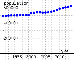
26.

This table and graph gives population estimates for Portland, Oregon from 1990 through 2014.

Year	Population	Year	Population
1990	487849	2003	539546
1991	491064	2004	533120
1992	493754	2005	534112
1993	497432	2006	538091
1994	497659	2007	546747
1995	498396	2008	556442
1996	501646	2009	566143
1997	503205	2010	585261
1998	502945	2011	593859
1999	503637	2012	602954
2000	529922	2013	609520
2001	535185	2014	619360
2002	538803

Between what two years that are two years apart was the rate of change highest?

What was that rate of change?

You have attempted of activities on this page.

Prev Top Next

\(x\) (input)	\(y\) (output)
\(1\)	\(2\)
\(2\)	\(4\)
\(3\)	\(6\)
\(5\)	\(10\)
\(10\)	\(20\)
Pattern: \(y=2x\)

\(x\)	\(y\)
\(0\)	\({10}\)
\(1\)	\({11}\)
\(2\)	\({12}\)
\(3\)	\({13}\)

\(x\)	\(y\)
\(0\)	\({-1}\)
\(1\)	\({2}\)
\(2\)	\({5}\)
\(3\)	\({8}\)

	\(x\)	\(y\)
	\(0\)	\({-1}\)
\({}+1\rightarrow\)	\(1\)	\({2}\)	\(\leftarrow{}+3\)
\({}+1\rightarrow\)	\(2\)	\({5}\)	\(\leftarrow{}+3\)
\({}+1\rightarrow\)	\(3\)	\({8}\)	\(\leftarrow{}+3\)

\(x\)	\(y\) using \(y=3x\)	Actual \(y\)
\(0\)	\(0\)	\({-1}\)
\(1\)	\(3\)	\({2}\)
\(2\)	\(6\)	\({5}\)
\(3\)	\(9\)	\({8}\)

\(x\)	\(y\)
\(-8\)	\(3.1\)
\(-5\)	\(2.1\)
\(-2\)	\(1.1\)
\(1\)	\(0.1\)

\(x\)	\(y\)
\(11\)	\(208\)
\(13\)	\(210\)
\(15\)	\(214\)
\(17\)	\(220\)

\(x\)	\(y\)
\(7\)	\({-2}\)
\(6\)	\({-3}\)
\(2\)	\({-7}\)
\(10\)	\({1}\)
\(16\)	\({7}\)

\(x\)	\(y\)
\(0.02\)	\({0.0004}\)
\(0.04\)	\({0.0016}\)
\(0.06\)	\({0.0036}\)
\(0.08\)	\({0.0064}\)
\(0.1\)	\({0.01}\)

\(x\)	\(y\)
\(0.07\)	\({0.0049}\)
\(0.1\)	\({0.01}\)
\(0.13\)	\({0.0169}\)
\(0.16\)	\({0.0256}\)
\(0.19\)	\({0.0361}\)

\(x\)	\(y\)
\(94\)	\({{\frac{1}{94}}}\)
\(62\)	\({{\frac{1}{62}}}\)
\(24\)	\({{\frac{1}{24}}}\)
\(4\)	\({{\frac{1}{4}}}\)
\(72\)	\({{\frac{1}{72}}}\)

\(x\)	\(y\)
\(8\)	\({65547}\)
\(9\)	\({262155}\)
\(10\)	\({1.04859\times 10^{6}}\)
\(11\)	\({4.19432\times 10^{6}}\)
\(12\)	\({1.67772\times 10^{7}}\)
\(13\)	\({6.71089\times 10^{7}}\)

\(x\)	\(y\)
\(6\)	\({{\frac{1}{6}}}\)
\(29\)	\({{\frac{1}{29}}}\)
\(67\)	\({{\frac{1}{67}}}\)
\(76\)	\({{\frac{1}{76}}}\)
\(71\)	\({{\frac{1}{71}}}\)

\(x\)	\(y\)
\(-2\)	\({49.43}\)
\(-1\)	\({44.93}\)
\(0\)	\({40.43}\)
\(1\)	\({35.93}\)
\(2\)	\({31.43}\)
\(3\)	\({26.93}\)