With the graph constructed we can now turn our attention to the algorithm we will use to find the shortest solution to the word ladder problem. The graph algorithm we are going to use is called the “breadth first search” algorithm. Breadth first search (BFS) is one of the easiest algorithms for searching a graph. It also serves as a prototype for several other important graph algorithms that we will study later.
Given a graph \(G\) and a starting vertex \(s\text{,}\) a breadth first search proceeds by exploring edges in the graph to find all the vertices in \(G\) for which there is a path from \(s\text{.}\) The remarkable thing about a breadth first search is that it finds all the vertices that are a distance \(k\) from \(s\) before it finds any vertices that are a distance \(k+1\text{.}\) One good way to visualize what the breadth first search algorithm does is to imagine that it is building a tree, one level of the tree at a time. A breadth first search adds all children of the starting vertex before it begins to discover any of the grandchildren.
To keep track of its progress, BFS colors each of the vertices white, gray, or black. All the vertices are initialized to white when they are constructed. A white vertex is an undiscovered vertex. When a vertex is initially discovered it is colored gray, and when BFS has completely explored a vertex it is colored black. This means that once a vertex is colored black, it has no white vertices adjacent to it. A gray node, on the other hand, may have some white vertices adjacent to it, indicating that there are still additional vertices to explore.
The breadth first search algorithm shown in Exploration 9.9.1 below uses the adjacency list graph representation we developed earlier. In addition it uses a Queue, a crucial point as we will see, to decide which vertex to explore next.
In addition the BFS algorithm uses an extended version of the Vertex class. This new vertex class adds three new instance variables: distance, predecessor, and color.
BFS begins at the starting vertex s and colors start gray to show that it is currently being explored. Two other values, the distance and the predecessor, are initialized to 0 and nullptr respectively for the starting vertex. Finally, start is placed on a Queue. The next step is to begin to systematically explore vertices at the front of the queue. We explore each new node at the front of the queue by iterating over its adjacency list. As each node on the adjacency list is examined its color is checked. If it is white, the vertex is unexplored, and four things happen:
nbr is added to the end of a queue. Adding nbr to the end of the queue effectively schedules this node for further exploration, but not until all the other vertices on the adjacency list of currentVert have been explored.
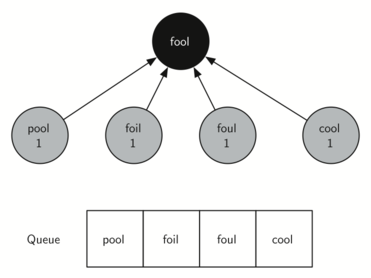
Let’s look at how the bfs function would construct the breadth first tree corresponding to the graph in Figure 9.8.1. Starting from fool we take all nodes that are adjacent to fool and add them to the tree. The adjacent nodes include pool, foil, foul, and cool. Each of these nodes are added to the queue of new nodes to expand. Figure 9.9.1 shows the state of the in-progress tree along with the queue after this step.
Image of a graph and a queue representing the first step in the breadth-first search algorithm. The graph has a central node labeled ’fool’, with arrows pointing to four connected nodes: ’pool’, ’foil’, a second ’foul’, and ’cool’, each marked with the number ’1’ to indicate a step or level. Below the graph, there’s a depiction of a queue with the words ’pool’, ’foil’, ’foul’, and ’cool’ enqueued in that order. This illustrates how the algorithm explores the neighbors of the starting node ’fool’ and adds them to the queue for further exploration.
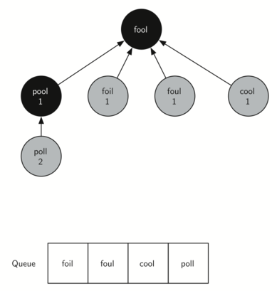
In the next step bfs removes the next node (pool) from the front of the queue and repeats the process for all of its adjacent nodes. However, when bfs examines the node cool, it finds that the color of cool has already been changed to gray. This indicates that there is a shorter path to cool and that cool is already on the queue for further expansion. The only new node added to the queue while examining pool is poll. The new state of the tree and queue is shown in Figure 9.9.2.
Image showing the second step in a breadth-first search algorithm on a word graph. The central node is labeled ’fool’, with connections to four adjacent nodes: ’pool’, ’foil’, ’foul’, and ’cool’, each marked with a ’1’ indicating they were reached in the first step of the search. ’Pool’ is further connected to a node labeled ’poll’, marked with a ’2’ indicating it is reached in the second step. Below the graph, a queue is shown containing ’foil’, ’foul’, ’cool’, and ’poll’, reflecting the order in which they are visited. This demonstrates the process of exploring each node’s neighbors and tracking the search progression through levels or layers.
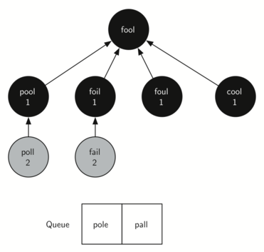
The next vertex on the queue is foil. The only new node that foil can add to the tree is fail. As bfs continues to process the queue, neither of the next two nodes add anything new to the queue or the tree. Figure 9.9.3 shows the tree and the queue after expanding all the vertices on the second level of the tree.
Image of a breadth-first search tree after completing one level. The tree starts at the top with the word ’fool’. Below ’fool’, there are four nodes labeled ’pool’, ’foil’, ’foul’, and ’cool’, each marked with the number ’1’. From ’foil’, there is an additional node labeled ’fail’, marked with the number ’2’. Similarly, ’pool’ connects to ’poll’, also marked with ’2’. The diagram indicates the sequence of words explored from the starting word ’fool’ by changing one letter at a time. Below the tree, there is a queue with the words ’pole’ and ’pall’, representing the next words to be visited in the search.
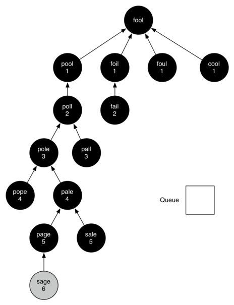
Image showing the final breadth-first search tree. The root of the tree is the word ’fool’ with four branches leading to the words ’pool’, ’foil’, ’foul’, and ’cool’, each marked with a ’1’ indicating the first level of connections. ’Pool’ connects to ’poll’ (level 2), which further connects to ’pole’ (level 3), leading to ’pope’ (level 4), then to ’page’ (level 5), and finally to ’sage’ (level 6). Similarly, ’foil’ connects to ’fail’ (level 2), and ’poll’ also connects to ’pall’ (level 3), leading to ’pale’ (level 4) and ’sale’ (level 5). The levels indicate the number of steps taken from the root word to reach each subsequent word by changing one letter at a time. An empty queue box is shown to the side, suggesting that the search has been completed.
You should continue to work through the algorithm on your own so that you are comfortable with how it works. Figure 9.9.4 shows the final breadth first search tree after all the vertices in Figure 9.9.1 have been expanded. The amazing thing about the breadth first search solution is that we have not only solved the FOOL–SAGE problem we started out with, but we have solved many other problems along the way. We can start at any vertex in the breadth first search tree and follow the predecessor arrows back to the root to find the shortest word ladder from any word back to fool. The function below (Listing 9.9.5) shows how to follow the predecessor links to print out the word ladder.
Listing 9.9.6 is a complete implementation of both the Vertex and Graph classes, along with an implementation for the breadth-first search shown above.