Section 9.15 General Depth First Search
The knight’s tour is a special case of a depth first search where the goal is to create the deepest depth first tree, without any branches. The more general depth first search is actually easier. Its goal is to search as deeply as possible, connecting as many nodes in the graph as possible and branching where necessary.
It is even possible that a depth first search will create more than one tree. When the depth first search algorithm creates a group of trees we call this a depth first forest. As with the breadth first search our depth first search makes use of predecessor links to construct the tree. In addition, the depth first search will make use of two additional instance variables in the
Vertex class. The new instance variables are the discovery and finish times. The discovery time tracks the number of steps in the algorithm before a vertex is first encountered. The finish time is the number of steps in the algorithm before a vertex is colored black. As we will see after looking at the algorithm, the discovery and finish times of the nodes provide some interesting properties we can use in later algorithms.
The code for our depth first search is shown in Listing 5. Since the two functions
dfs and its helper dfsvisit use a variable to keep track of the time across calls to dfsvisit we chose to implement the code as methods of a class that inherits from the Graph class. This implementation extends the graph class by adding a time instance variable and the two methods dfs and dfsvisit. Looking at line 11 you will notice that the dfs method iterates over all of the vertices in the graph calling dfsvisit on the nodes that are white. The reason we iterate over all the nodes, rather than simply searching from a chosen starting node, is to make sure that all nodes in the graph are considered and that no vertices are left out of the depth first forest. It may look unusual to see the statement for aVertex in self, but remember that in this case self is an instance of the DFSGraph class, and iterating over all the vertices in an instance of a graph is a natural thing to do.
Although our implementation of
bfs was only interested in considering nodes for which there was a path leading back to the start, it is possible to create a breadth first forest that represents the shortest path between all pairs of nodes in the graph. We leave this as an exercise. In our next two algorithms we will see why keeping track of the depth first forest is important.
The
dfsvisit method starts with a single vertex called startVertex and explores all of the neighboring white vertices as deeply as possible. If you look carefully at the code for dfsvisit and compare it to breadth first search, what you should notice is that the dfsvisit algorithm is almost identical to bfs except that on the last line of the inner for loop, dfsvisit calls itself recursively to continue the search at a deeper level, whereas bfs adds the node to a queue for later exploration. It is interesting to note that where bfs uses a queue, dfsvisit uses a stack. You don’t see a stack in the code, but it is implicit in the recursive call to dfsvisit.
The following sequence of figures illustrates the depth first search algorithm in action for a small graph. In these figures, the dotted lines indicate edges that are checked, but the node at the other end of the edge has already been added to the depth first tree. In the code this test is done by checking that the color of the other node is non-white.
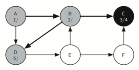
The search begins at vertex A of the graph (Figure 9.15.1). Since all of the vertices are white at the beginning of the search the algorithm visits vertex A. The first step in visiting a vertex is to set the color to gray, which indicates that the vertex is being explored and the discovery time is set to 1. Since vertex A has two adjacent vertices (B, D) each of those need to be visited as well. We’ll make the arbitrary decision that we will visit the adjacent vertices in alphabetical order.
Vertex B is visited next (Figure 9.15.2), so its color is set to gray and its discovery time is set to 2. Vertex B is also adjacent to two other nodes (C, D) so we will follow the alphabetical order and visit node C next.
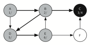
Visiting vertex C (Figure 9.15.3) brings us to the end of one branch of the tree. After coloring the node gray and setting its discovery time to 3, the algorithm also determines that there are no adjacent vertices to C. This means that we are done exploring node C and so we can color the vertex black, and set the finish time to 4. You can see the state of our search at this point in Figure 9.15.4.
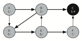
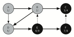
Since vertex C was the end of one branch we now return to vertex B and continue exploring the nodes adjacent to B. The only additional vertex to explore from B is D, so we can now visit D (Figure 9.15.5) and continue our search from vertex D. Vertex D quickly leads us to vertex E (Figure 9.15.6). Vertex E has two adjacent vertices, B and F. Normally we would explore these adjacent vertices alphabetically, but since B is already colored gray the algorithm recognizes that it should not visit B since doing so would put the algorithm in a loop! So exploration continues with the next vertex in the list, namely F (Figure 9.15.7).
Vertex F has only one adjacent vertex, C, but since C is colored black there is nothing else to explore, and the algorithm has reached the end of another branch. From here on, you will see in Figure 9.15.8 through Figure 9.15.12 that the algorithm works its way back to the first node, setting finish times and coloring vertices black.
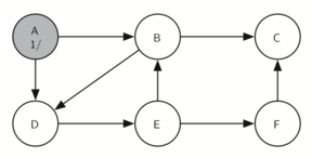
A graph with six nodes labeled A through F. Node A is marked as the starting point with a ’1’ and has directed edges to nodes B and D, showing the initial branching in a depth-first search tree.
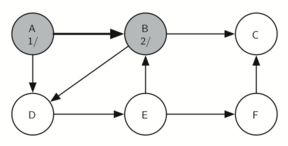
The graph extends from Figure 14, showing node B as the next node visited in the search, indicated by a ’2’. Nodes E and C are shown as subsequent nodes, but not yet visited.
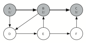
Continuing the sequence, node C is now marked with a ’3’, showing the progression of the depth-first search moving to the next unvisited node in the tree.
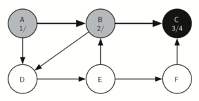
The graph further expands with node C’s child nodes, marked as ’3/4’, indicating the depth-first search is exploring the deeper levels of the tree
Depth-first search progression with node D marked ’5’, indicating its visit after nodes A, B, and C, and before node E.
Node E is visited, labeled ’6’ in the search sequence, following the exploration from node D in the depth-first search tree.
The search continues with node F now visited, labeled with ’7’, and an unvisited node is connected to node C with a directed edge.
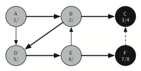
The final stage of the depth-first search, with nodes F and B marked as ’7/8’, showing the completion of the tree traversal.
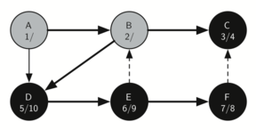
A depth-first search tree diagram with nodes A to F, where nodes A, B, and C are sequentially numbered 1 to 3/4, and nodes D, E, and F are numbered 5, 6, and 7/8 respectively, showing the order of traversal.
Continuation of the depth-first search tree, with node E now having two numbers, 6/9, indicating the backtracking process and further search.
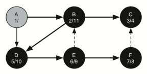
Further progress in the depth-first search tree, node B is now numbered 2/11, showing that the search has returned to this node after exploring other branches.
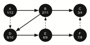
The final stage in the depth-first search process with node A labeled as 1/12, completing the full traversal of the search tree.
The starting and finishing times for each node display a property called the parenthesis property. This property means that all the children of a particular node in the depth first tree have a later discovery time and an earlier finish time than their parent. Figure 9.15.13 shows the tree constructed by the depth first search algorithm.
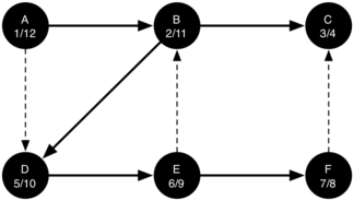
A completed depth first search tree with six nodes labeled A to F. The nodes are interconnected with arrows indicating the path of the search. Each node is annotated with two numbers; the first number represents the order in which the node was first visited, and the second number represents the order in which the final visit occurred, marking the node’s completion in the search. Node A is labeled "1/12", B "2/11", C "3/4", D "5/10", E "6/9", and F "7/8". This indicates the starting point of the search at node A, the backtracking steps, and the overall path taken to explore all the nodes.
The visualization in Figure 9.15.14 shows the entire traversal of the example graph shown above. Nodes attached to an orange line are connected to the node attached with a brown line. This relationship is directional, and mirrors what can be observed above.
You have attempted of activities on this page.
