7.5. The Insertion Sort
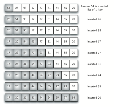
The insertion sort, although still \(O(n^{2})\), works in a slightly different way. It always maintains a sorted subvector in the lower positions of the vector. Each new item is then “inserted” back into the previous subvector such that the sorted subvector is one item larger. Figure 4 shows the insertion sorting process. The shaded items represent the ordered subvectors as the algorithm makes each pass.

Figure 4: insertionSort
We begin by assuming that a vector with one item (position \(0\)) is already sorted. On each pass, one for each item 1 through \(n-1\), the current item is checked against those in the already sorted subvector. As we look back into the already sorted subvector, we shift those items that are greater to the right. When we reach a smaller item or the end of the subvector, the current item can be inserted.
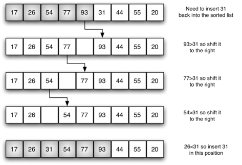
Figure 5 shows the fifth pass in detail. At this point in the algorithm, a sorted subvector of five items consisting of 17, 26, 54, 77, and 93 exists. We want to insert 31 back into the already sorted items. The first comparison against 93 causes 93 to be shifted to the right. 77 and 54 are also shifted. When the item 26 is encountered, the shifting process stops and 31 is placed in the open position. Now we have a sorted subvector of six items.

Figure 5: insertionSort: Fifth Pass of the Sort
The implementation of insertionSort (ActiveCode 1) shows that
there are again \(n-1\) passes to sort n items. The iteration
starts at position 1 and moves through position \(n-1\), as these
are the items that need to be inserted back into the sorted subvectors.
Line 8 performs the shift operation that moves a value up one position
in the vector, making room behind it for the insertion. Remember that this
is not a complete exchange as was performed in the previous algorithms.
The maximum number of comparisons for an insertion sort is the sum of the first \(n-1\) integers. Again, this is \(O(n^{2})\). However, in the best case, only one comparison needs to be done on each pass. This would be the case for an already sorted vector.
One note about shifting versus exchanging is also important. In general, a shift operation requires approximately a third of the processing work of an exchange since only one assignment is performed. In benchmark studies, insertion sort will show very good performance.
The visualization above allows you to step through the algorithm. Red bars represent the element being looked at and blue represents the last element to look at during a pass.
The visualization below allows you to examine the individual steps of the algorithm at a slower pace. Bars that are orange indicate that it is being compared to items to the left. Bars that are blue indicate that it is one of the items currently being compared against the orange bar.
Self Check
- Q-5: Suppose you have the following list of numbers to sort:
[15, 5, 4, 18, 12, 19, 14, 10, 8, 20] which list represents the partially sorted list after three complete passes of insertion sort?
- [4, 5, 12, 15, 14, 10, 8, 18, 19, 20]
- This is the result of bubble sort.
- [15, 5, 4, 10, 12, 8, 14, 18, 19, 20]
- This is the result of selection sort.
- [4, 5, 15, 18, 12, 19, 14, 10, 8, 20]
- Insertion sort works at the start of the list. Each pass produces a longer sorted list.
- [15, 5, 4, 18, 12, 19, 14, 8, 10, 20]
- Insertion sort works on the front of the list not the end.