
9.7. Fractals and Percolation Models
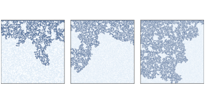
Figure 9.8: Percolation models with q=0.6 and n=100, 200, and 300.
Now let’s get back to percolation models. Figure 9.8 shows clusters of wet cells in percolation simulations with p=0.6 and n=100, 200, and 300. Informally, they resemble fractal patterns seen in nature and in mathematical models.
To estimate their fractal dimension, we can run CAs with a range of sizes, count the number of wet cells in each percolating cluster, and then see how the cell counts scale as we increase the size of the array.
The following loop runs the simulations:
res = []
for size in sizes:
    perc = Percolation(size, q)
    if test_perc(perc):
        num_filled = perc.num_wet() - size
        res.append((size, size**2, num_filled))
The result is a list of tuples where each tuple contains size, size**2, and the number of cells in the percolating cluster (not including the initial wet cells in the top row).
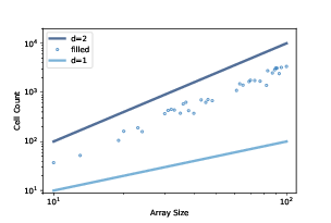
Figure 9.9: Number of cells in the percolating cluster versus CA size.
Figure 9.9 shows the results for a range of sizes from 10 to 100. The dots show the number of cells in each percolating cluster. The slope of a line fitted to these dots is often near 1.85, which suggests that the percolating cluster is, in fact, fractal when q is near the critical value.
When q is larger than the critical value, nearly every porous cell gets filled, so the number of wet cells is close to \(q * size^2\), which has dimension 2.
When q is substantially smaller than the critical value, the number of wet cells is proportional to the linear size of the array, so it has dimension 1.
- When the value q is larger than the critical value
- Correct!
- When the value q is smaller than the critical value
- No, this would mean that the number of wet cells is proportional to the linear size of the array, so it has dimension 1.
- When the value q is the same as the critical value
- Not quite, this would not typically happen.
- When the value q is near the critical value.
- No, this suggests that the percolating cluster is, in fact, fractal.
Q-1: When is a graph dimension 2?