
11.4. Segregation
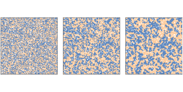
Figure 11.1: Schelling’s segregation model with n=100, initial condition (left), after 2 steps (middle), and after 10 steps (right).
Now let’s see what happens when we run the model, starting with n=100 and p=0.3, and run for 10 steps.
grid = Schelling(n=100, p=0.3)
for i in range(10):
    grid.step()
Figure 11.1 shows the initial configuration (left), the state of the simulation after 2 steps (middle), and the state after 10 steps (right).
Clusters form almost immediately and grow quickly, until most agents live in highly-segregated neighborhoods.
As the simulation runs, we can compute the degree of segregation, which is the average, across agents, of the fraction of neighbors who are the same color as the agent:
np.nanmean(frac_same)
In Figure 11.1, the average fraction of similar neighbors is 50% in the initial configuration, 65% after two steps, and 76% after 10 steps!
Remember that when p=0.3 the agents would be happy if 3 of 8 neighbors were their own color, but they end up living in neighborhoods where 6 or 7 of their neighbors are their own color, typically.
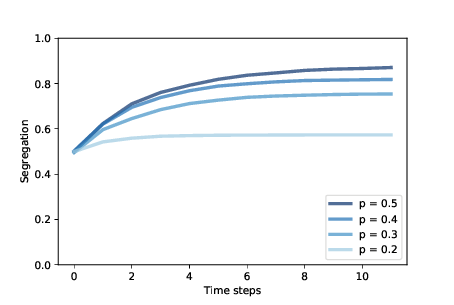
Figure 11.2: Degree of segregation in Schelling’s model, over time, for a range of p.
Figure 11.2 shows how the degree of segregation increases and where it levels off for several values of p. When p=0.4, the degree of segregation in steady state is about 82%, and a majority of agents have no neighbors with a different color.
These results are surprising to many people, and they make a striking example of the unpredictable relationship between individual decisions and system behavior.
- 30%
- Sorry but that is what percentage of agents will be unhappy if p=0.3.
- 82%
- Correct!
- 76%
- Sorry but that was the percentage from 10 steps into the p=0.3 example above.
- 50%
- Sorry but that was the initial configuration of the p=0.3 example above.
Q-2: When p=0.4 what is the approximate degree of segregation in a steady state?