Logo image

Active Calculus

Section 3.2 Using derivatives to describe families of functions

Mathematicians are often interested in making general observations, say by describing patterns that hold in a large number of cases. Think about the Pythagorean Theorem: it doesn’t tell us something about a single right triangle, but rather a fact about every right triangle. In the next part of our studies, we use calculus to make general observations about families of functions that depend on one or more parameters. People who use applied mathematics, such as engineers and economists, often encounter the same types of functions where only small changes to certain constants occur. These constants are called parameters.
Figure 3.2.1. The graph of \(f(t) = a \sin(b(t-c)) + d\) based on parameters \(a\text{,}\) \(b\text{,}\) \(c\text{,}\) and \(d\text{.}\)
You are already familiar with certain families of functions. For example, \(f(t) = a \sin(b(t-c)) + d\) is a stretched and shifted version of the sine function with amplitude \(a\text{,}\) period \(\frac{2\pi}{b}\text{,}\) phase shift \(c\text{,}\) and vertical shift \(d\text{.}\) We know that \(a\) affects the size of the oscillation, \(b\) the rapidity of oscillation, and \(c\) where the oscillation starts, as shown in Figure 3.2.1, while \(d\) affects the vertical positioning of the graph.
As another example, every function of the form \(y = mx + b\) is a line with slope \(m\) and \(y\)-intercept \((0,b)\text{.}\) The value of \(m\) affects the line’s steepness, and the value of \(b\) situates the line vertically on the coordinate axes. These two parameters describe all possible non-vertical lines.
For other less familiar families of functions, we can use calculus to discover where key behavior occurs: where members of the family are increasing or decreasing, concave up or concave down, where relative extremes occur, and more, all in terms of the parameters involved. To get started, we revisit a common collection of functions to see how calculus confirms things we already know.

Preview Activity 3.2.1.

Let \(a\text{,}\) \(h\text{,}\) and \(k\) be arbitrary real numbers with \(a \ne 0\text{,}\) and let \(f\) be the function given by the rule \(f(x) = a(x-h)^2 + k\text{.}\)
  1. What familiar type of function is \(f\text{?}\) What information do you know about \(f\) just by looking at its form? (Think about the roles of \(a\text{,}\) \(h\text{,}\) and \(k\text{.}\))
  2. Next we use some calculus to develop familiar ideas from a different perspective. To start, treat \(a\text{,}\) \(h\text{,}\) and \(k\) as constants and compute \(f'(x)\text{.}\)
  3. Find all critical numbers of \(f\text{.}\) (These will depend on at least one of \(a\text{,}\) \(h\text{,}\) and \(k\text{.}\))
  4. Assume that \(a \lt 0\text{.}\) Construct a first derivative sign chart for \(f\text{.}\)
  5. Based on the information you’ve found above, classify the critical values of \(f\) as maxima or minima.

Subsection 3.2.1 Describing families of functions in terms of parameters

Our goal is to describe the key characteristics of the overall behavior of each member of a family of functions in terms of its parameters. By finding the first and second derivatives and constructing sign charts (each of which may depend on one or more of the parameters), we can often make broad conclusions about how each member of the family will appear.

Example 3.2.2.

Consider the two-parameter family of functions given by \(g(x) = axe^{-bx}\text{,}\) where \(a\) and \(b\) are positive real numbers. Fully describe the behavior of a typical member of the family in terms of \(a\) and \(b\text{,}\) including the location of all critical numbers, where \(g\) is increasing, decreasing, concave up, and concave down, and the long term behavior of \(g\text{.}\)
Solution.
We begin by computing \(g'(x)\text{.}\) By the product rule,
\begin{equation*} g'(x) = ax \frac{d}{dx}\left[e^{-bx}\right] + e^{-bx} \frac{d}{dx}[ax]\text{.} \end{equation*}
By applying the chain rule and constant multiple rule, we find that
\begin{equation*} g'(x) = axe^{-bx}(-b) + e^{-bx}(a)\text{.} \end{equation*}
To find the critical numbers of \(g\text{,}\) we solve the equation \(g'(x) = 0\text{.}\) By factoring \(g'(x)\text{,}\) we find
\begin{equation*} 0 = ae^{-bx}(-bx + 1)\text{.} \end{equation*}
Since we are given that \(a \ne 0\) and we know that \(e^{-bx} \ne 0\) for all values of \(x\text{,}\) the only way this equation can hold is when \(-bx + 1 = 0\text{.}\) Solving for \(x\text{,}\) we find \(x = \frac{1}{b}\text{,}\) and this is therefore the only critical number of \(g\text{.}\)
We construct the first derivative sign chart for \(g\) that is shown in Figure 3.2.3.
Figure 3.2.3. The first derivative sign chart for \(g(x) = axe^{-bx}\text{.}\)
Because the factor \(ae^{-bx}\) is always positive, the sign of \(g'\) depends on the linear factor \((1-bx)\text{,}\) which is positive for \(x \lt \frac{1}{b}\) and negative for \(x \gt \frac{1}{b}\text{.}\) Hence we can not only conclude that \(g\) is always increasing for \(x \lt \frac{1}{b}\) and decreasing for \(x \gt \frac{1}{b}\text{,}\) but also that \(g\) has a global maximum at \((\frac{1}{b}, g(\frac{1}{b}))\) and no local minimum.
We turn next to analyzing the concavity of \(g\text{.}\) With \(g'(x) = -abxe^{-bx} + ae^{-bx}\text{,}\) we differentiate to find that
\begin{equation*} g''(x) = -abxe^{-bx}(-b) + e^{-bx}(-ab) + ae^{-bx}(-b)\text{.} \end{equation*}
Combining like terms and factoring, we now have
\begin{equation*} g''(x) = ab^2xe^{-bx} - 2abe^{-bx} = abe^{-bx}(bx - 2)\text{.} \end{equation*}
Figure 3.2.4. The second derivative sign chart for \(g(x) = axe^{-bx}\text{.}\)
We observe that \(abe^{-bx}\) is always positive, and thus the sign of \(g''\) depends on the sign of \((bx-2)\text{,}\) which is zero when \(x = \frac{2}{b}\text{.}\) Since \(b\) is positive, the value of \((bx-2)\) is negative for \(x \lt \frac{2}{b}\) and positive for \(x \gt \frac{2}{b}\text{.}\) The sign chart for \(g''\) is shown in Figure 3.2.4. Thus, \(g\) is concave down for all \(x \lt \frac{2}{b}\) and concave up for all \(x \gt \frac{2}{b}\text{.}\)
Finally, we analyze the long term behavior of \(g\) by considering two limits. First, we note that
\begin{equation*} \lim_{x \to \infty} g(x) = \lim_{x \to \infty} axe^{-bx} = \lim_{x \to \infty} \frac{ax}{e^{bx}}\text{.} \end{equation*}
This limit has indeterminate form \(\frac{\infty}{\infty}\text{,}\) so we apply L’Hôpital’s Rule and find that \(\lim_{x \to \infty} g(x) = 0\text{.}\) In the other direction,
\begin{equation*} \lim_{x \to -\infty} g(x) = \lim_{x \to -\infty} axe^{-bx} = -\infty\text{,} \end{equation*}
because \(ax \to -\infty\) and \(e^{-bx} \to \infty\) as \(x \to -\infty\text{.}\) Hence, as we move left on its graph, \(g\) decreases without bound, while as we move to the right, \(g(x) \to 0\text{.}\)
All of this information now helps us produce the graph of a typical member of this family of functions without using a graphing utility (and without choosing particular values for \(a\) and \(b\)), as shown in Figure 3.2.5.
Figure 3.2.5. The graph of \(g(x) = axe^{-bx}\text{.}\)
Note that the value of \(b\) controls the horizontal location of the global maximum and the inflection point, as neither depends on \(a\text{.}\) The value of \(a\) affects the vertical stretch of the graph. For example, the global maximum occurs at the point \((\frac{1}{b}, g(\frac{1}{b})) = (\frac{1}{b}, \frac{a}{b}e^{-1})\text{,}\) so the larger the value of \(a\text{,}\) the greater the value of the global maximum.
The work we’ve completed in Example 3.2.2 can often be replicated for other families of functions that depend on parameters. Normally we are most interested in determining all critical numbers, a first derivative sign chart, a second derivative sign chart, and the limit of the function as \(x \to \infty\text{.}\) Throughout, we prefer to work with the parameters as arbitrary constants. In addition, we can experiment with some particular values of the parameters present to reduce the algebraic complexity of our work. The following activities offer several key examples where we see that the values of the parameters substantially affect the behavior of individual functions within a given family.

Activity 3.2.2.

Consider the family of functions defined by \(p(x) = x^3 - ax\text{,}\) where \(a \ne 0\) is an arbitrary constant.
  1. Find \(p'(x)\) and determine the critical numbers of \(p\text{.}\) How many critical numbers does \(p\) have?
  2. Construct a first derivative sign chart for \(p\text{.}\) What can you say about the overall behavior of \(p\) if the constant \(a\) is positive? Why? What if the constant \(a\) is negative? In each case, describe the relative extremes of \(p\text{.}\)
  3. Find \(p''(x)\) and construct a second derivative sign chart for \(p\text{.}\) What does this tell you about the concavity of \(p\text{?}\) What role does \(a\) play in determining the concavity of \(p\text{?}\)
  4. Without using a graphing utility, sketch and label typical graphs of \(p(x)\) for the cases where \(a\gt 0\) and \(a \lt 0\text{.}\) Label all inflection points and local extrema.
  5. Finally, use a graphing utility to test your observations above by entering and plotting the function \(p(x) = x^3 - ax\) for at least four different values of \(a\text{.}\) Write several sentences to describe your overall conclusions about how the behavior of \(p\) depends on \(a\text{.}\)
Hint.
  1. When solving \(p'(x) = 0\text{,}\) think about two possible cases: when \(a\gt 0\) and when \(a \lt 0\text{.}\)
  2. Remember that any quadratic function can be zero at most two times. How does the graph of \(y = 3x^2 - a\) look?
  3. Don’t forget that \(\frac{d}{dx}[a] = 0\text{.}\)
  4. Think about how a typical cubic polynomial’s graph behaves.

Activity 3.2.3.

Consider the two-parameter family of functions of the form \(h(x) = a(1-e^{-bx})\text{,}\) where \(a\) and \(b\) are positive real numbers.
  1. Find the first derivative and the critical numbers of \(h\text{.}\) Use these to construct a first derivative sign chart and determine for which values of \(x\) the function \(h\) is increasing and decreasing.
  2. Find the second derivative and build a second derivative sign chart. For which values of \(x\) is a function in this family concave up? concave down?
  3. What is the value of \(\lim_{x \to \infty} a(1-e^{-bx})\text{?}\) \(\lim_{x \to -\infty} a(1-e^{-bx})\text{?}\)
  4. How does changing the value of \(b\) affect the shape of the curve?
  5. Without using a graphing utility, sketch the graph of a typical member of this family. Write several sentences to describe the overall behavior of a typical function \(h\) and how this behavior depends on \(a\) and \(b\text{.}\)
Hint.
  1. Expand to write \(h(x) = a - ae^{-bx}\) before differentiating.
  2. Remember that \(e^{-bx}\) is never zero and always positive, regardless of the value of \(x\text{.}\)
  3. Recall that \(e^{-x} \to 0\) as \(x \to \infty\) and \(e^{-x} \to \infty\) as \(x \to -\infty\text{.}\)
  4. Consider how \(b\) affects the value of \(h'(x)\text{.}\)
  5. Use your work in (a)-(d).

Activity 3.2.4.

Let \(L(t) = \frac{A}{1+ce^{-kt}}\text{,}\) where \(A\text{,}\) \(c\text{,}\) and \(k\) are all positive real numbers.
  1. Observe that we can equivalently write \(L(t) = A(1+ce^{-kt})^{-1}\text{.}\) Find \(L'(t)\) and explain why \(L\) has no critical numbers. Is \(L\) always increasing or always decreasing? Why?
  2. Given the fact that
    \begin{equation*} L''(t) = Ack^2e^{-kt} \frac{ce^{-kt}-1}{(1+ce^{-kt})^3}\text{,} \end{equation*}
    find all values of \(t\) such that \(L''(t) = 0\) and hence construct a second derivative sign chart. For which values of \(t\) is a function in this family concave up? concave down?
  3. What is the value of \(\lim_{t \to \infty} \frac{A}{1+ce^{-kt}}\text{?}\) \(\lim_{t \to -\infty} \frac{A}{1+ce^{-kt}}\text{?}\)
  4. Find the value of \(L(x)\) at the inflection point found in (b).
  5. Without using a graphing utility, sketch the graph of a typical member of this family. Write several sentences to describe the overall behavior of a typical function \(L\) and how this behavior depends on \(A\text{,}\) \(c\text{,}\) and \(k\) number.
  6. Explain why it is reasonable to think that the function \(L(t)\) models the growth of a population over time in a setting where the largest possible population the surrounding environment can support is \(A\text{.}\)
Hint.
  1. Use the chain rule, treating \(A\text{,}\) \(c\text{,}\) and \(k\) as constants.
  2. Note that the only way \(L''(t) = 0\) is if \(ce^{-kt}-1 = 0\text{.}\)
  3. Remember that \(e^{-t} \to 0\) as \(t \to \infty\) and \(e^{-t} \to \infty\) as \(t \to -\infty\text{.}\)
  4. Don’t forget that \(e^{\ln(x)} = x\) for all \(x \gt 0\text{.}\)
  5. Think about horizontal asymptotes, where \(L\) is increasing and decreasing, and concavity.

Subsection 3.2.2 Summary

  • Given a family of functions that depends on one or more parameters, by investigating how critical numbers and locations where the second derivative is zero depend on the values of these parameters, we can often accurately describe the shape of the function in terms of the parameters.
  • In particular, just as we can created first and second derivative sign charts for a single function, we often can do so for entire families of functions where critical numbers and possible inflection points depend on arbitrary constants. These sign charts then reveal where members of the family are increasing or decreasing, concave up or concave down, and help us to identify relative extremes and inflection points.

Exercises 3.2.3 Exercises

1. Drug dosage with a parameter.

For some positive constant \(C\text{,}\) a patient’s temperature change, \(T\text{,}\) due to a dose, \(D\text{,}\) of a drug is given by \(T = \left(\frac{C}{2} - \frac{D}{3}\right)D^2.\)
What dosage maximizes the temperature change?
\(D =\)
The sensitivity of the body to the drug is defined as \(dT/dD\text{.}\) What dosage maximizes sensitivity?
\(D =\)

2. Using the graph of \(g'\).

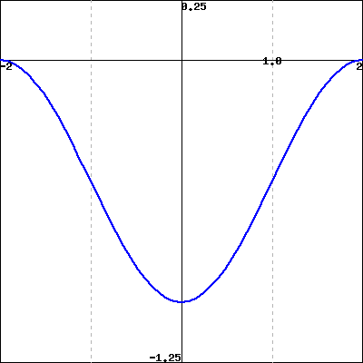
The figure below gives the behavior of the derivative of \(g(x)\) on \(-2\le x\le 2\text{.}\)
Graph of \(g'(x)\) (not \(g(x)\))
(Click on the graph to get a larger version.)
Sketch a graph of \(g(x)\) and use your sketch to answer the following questions.
A. Where does the graph of \(g(x)\) have inflection points?
\(x =\)
Enter your answer as a comma-separated list of values, or enter none if there are none.
B. Where are the global maxima and minima of \(g\) on \([-2,2]\text{?}\)
minimum at \(x =\)
maximum at \(x =\)
C. If \(g(-2) = -8\text{,}\) what are possible values for \(g(0)\text{?}\)
\(g(0)\) is in
(Enter your answer as an interval, or union of intervals, giving the possible values. Thus if you know \(-5 \lt g(0) \le -2\text{,}\) enter (-5,-2]. Enter infinity for \(\infty\text{,}\) the interval [1,1] to indicate a single point).
How is the value of \(g(2)\) related to the value of \(g(0)\text{?}\)
\(g(2)\) \(g(0)\)
(Enter the appropriate mathematical equality or inequality, \(=\text{,}\) \(\lt \text{,}\) \(>\text{,}\) etc.)

3.

Consider the one-parameter family of functions given by \(p(x) = x^3-ax^2\text{,}\) where \(a \gt 0\text{.}\)
  1. Sketch a plot of a typical member of the family, using the fact that each is a cubic polynomial with a repeated zero at \(x = 0\) and another zero at \(x = a\text{.}\)
  2. Find all critical numbers of \(p\text{.}\)
  3. Compute \(p''\) and find all values for which \(p''(x) = 0\text{.}\) Hence construct a second derivative sign chart for \(p\text{.}\)
  4. Describe how the location of the critical numbers and the inflection point of \(p\) change as \(a\) changes. That is, if the value of \(a\) is increased, what happens to the critical numbers and inflection point?

4.

Let \(q(x) = \frac{e^{-x}}{x-c}\) be a one-parameter family of functions where \(c \gt 0\text{.}\)
  1. Explain why \(q\) has a vertical asymptote at \(x = c\text{.}\)
  2. Determine \(\lim_{x \to \infty} q(x)\) and \(\lim_{x \to -\infty} q(x)\text{.}\)
  3. Compute \(q'(x)\) and find all critical numbers of \(q\text{.}\)
  4. Construct a first derivative sign chart for \(q\) and determine whether each critical number leads to a local minimum, local maximum, or neither for the function \(q\text{.}\)
  5. Sketch a typical member of this family of functions with important behaviors clearly labeled.

5.

Let \(E(x) = e^{-\frac{(x-m)^2}{2s^2}}\text{,}\) where \(m\) is any real number and \(s\) is a positive real number.
  1. Compute \(E'(x)\) and hence find all critical numbers of \(E\text{.}\)
  2. Construct a first derivative sign chart for \(E\) and classify each critical number of the function as a local minimum, local maximum, or neither.
  3. It can be shown that \(E''(x)\) is given by the formula
    \begin{equation*} E''(x) = e^{-\frac{(x-m)^2}{2s^2}} \left(\frac{(x-m)^2 - s^2}{s^4} \right)\text{.} \end{equation*}
    Find all values of \(x\) for which \(E''(x) = 0\text{.}\)
  4. Determine \(\lim_{x \to \infty} E(x)\) and \(\lim_{x \to -\infty} E(x)\text{.}\)
  5. Construct a labeled graph of a typical function \(E\) that clearly shows how important points on the graph of \(y = E(x)\) depend on \(m\) and \(s\text{.}\)
You have attempted of activities on this page.