Appendix A Answers to Activities

This appendix contains answers to all activities in the text. Answers for preview activities are not included.

1 Relating Changing Quantities
1.1 Changing in Tandem
1.1.2 Using Graphs to Represent Relationships


Activity 1.1.2.

1.1.2.a
Answer.
Sketches should look something like the following image.
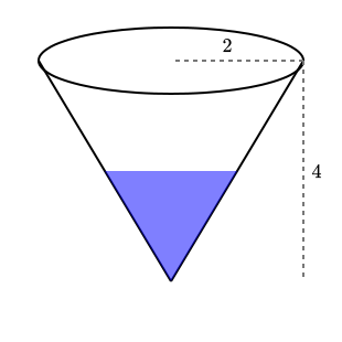
described in detail following the image
An inverted cone with labeled radius \(2\) ft and depth \(4\) ft, with water partially filling the bottom of the tank.
1.1.2.b
Answer.
Changing: volume, height, surface area, and time. Not changing: rate of water entering, height of tank, and radius of tank.
1.1.2.c
Answer.
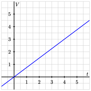
\(t\) \(V\)
\(0\) \(0\)
\(1\) \(0.75\)
\(2\) \(1.5\)
\(3\) \(2.25\)
\(4\) \(3.0\)
\(5\) \(3.75\)
described in detail following the image
A graph of volume versus time, using the values from the table. The graph is a straight line through the origin with slope \(0.75\text{.}\)
1.1.2.d
Answer.
Sketches should show a curve starting at the origin that is bending downwards as it approaches the maximum depth of \(4\) ft.
1.1.3 Using Algebra to Add Perspective


Activity 1.1.3.

1.1.3.a
Answer.
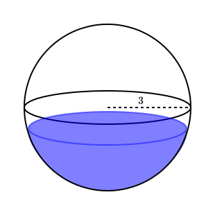
Sketches should look something like the following image.
described in detail following the image
An sphere with labeled radius \(3\) ft, with water partially filling the bottom of the spherical tank.
1.1.3.b
Answer.
Changing: volume, height, surface area, and time. Not changing: rate of water being pumped out and radius of the tank.
1.1.3.e
Answer.
\(t\) \(V\)
\(0\) \(113.1\)
\(20\) \(89.1\)
\(40\) \(65.1\)
\(60\) \(41.1\)
\(80\) \(17.1\)
\(94.25\) \(0\)
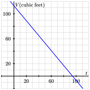
described in detail following the image
A graph of volume versus time, using the values from the table. The graph is a straight line through \((0, 36\pi)\) with slope \(-1.2\text{.}\)
1.1.3.f
Answer.
Sketches should show an S-shaped decreasing curve from \(h = 6\) to \(h = 0\text{.}\)

1.2 Functions: Modeling Relationships
1.2.2 Functions


Activity 1.2.2.

1.2.2.b
Answer.
The domain is \([0, 8]\) and the codomain is \(\left[0, \frac{256\pi}{3}\right]\text{.}\)
1.2.2.c
Answer.
\begin{align*} f(2)\amp = \frac{40\pi}{3} \approx 41.9 \text{ m}^3\\ f(4)\amp = \frac{128\pi}{3} \approx 134.0 \text{ m}^3\\ f(8)\amp = \frac{256\pi}{3} \approx 268.1 \text{ m}^3 \end{align*}

1.2.3 Comparing models and abstract functions


Activity 1.2.3.

1.2.3.a
Answer.
At \(t = 0\text{,}\) the height of the water is \(8\) m. At \(t = 1\) minute, the height is \(7.5\) m. At \(t = 2\) minutes, the height is \(7\) m. It will take \(16\) minutes for the tank to drain completely.
1.2.3.b
Answer.
The domain of each model is \(0 \le t \le 16\text{,}\) or equivalently \([0, 16]\text{.}\)
1.2.3.c
Answer.
When the tank is full, there are \(\frac{256\pi}{3} \approx 268.1\) cubic meters of water in the tank. The range of the model \(h = q(t)\) is \(0 \le h \le 8\text{,}\) or equivalently \([0, 8]\text{.}\) The range of the model \(V = p(t)\) is \(0 \le V \le \frac{256\pi}{3}\text{,}\) or equivalently \(\left[0, \frac{256\pi}{3}\right]\text{.}\)
1.2.3.d
Answer.
Descriptions will vary. The graph of \(V = p(t) = \frac{256\pi}{3} - \frac{\pi}{24}t^2(24-t)\) on \([0,16]\) is a curve that decreases from \(V(0) = \frac{256\pi}{3} \approx 268\) cubic meters down to \(V(16) = 0\text{.}\) The domain is \([0, 16]\) minutes and the range is \(\left[0, \frac{256\pi}{3}\right]\) cubic meters.
1.2.3.e
Answer.
The model’s domain is restricted to \([0, 16]\) and its range to \(\left[0, \frac{256\pi}{3}\right]\) by the physical context. The abstract function has an unrestricted domain and an unrestricted range.
1.2.3.f
Answer.
The height function should be linear and decreasing. The formula is \(q(t) = 8 - 0.5t.\)

1.2.4 Determining whether a relationship is a function or not


Activity 1.2.4.

1.2.4.a
Answer.
The circle is not a function of \(x\text{,}\) but the curve in the right-hand figure is a function of \(x\text{.}\)
1.2.4.b
Answer.
The relationship between the day of the year and the S&P500 stock index is a function.
1.2.4.d
Answer.
Not a function, because there is at least one input value which corresponds to more than one output value.

1.3 The Average Rate of Change of a Function
1.3.2 Defining and interpreting the average rate of change of a function


Activity 1.3.2.

1.3.2.a
Answer.
For Kent County, \(AV_{[1990,2010]} \approx 5099.55\) people per year. For Ottawa County, \(AV_{[1990,2010]} \approx 3801.65\) people per year.
1.3.2.c
Answer.
In an average year between 1990 and 2010, the population of Ottawa County was increasing by approximately 3801.65 people per year.
1.3.2.d
Answer.
Kent County had a greater average rate of change during the time interval \([2000,2010]\text{.}\) There were no intervals in which either county had a negative average rate of change.

1.3.3 How average rate of change indicates function trends


Activity 1.3.3.

1.3.3.a
Answer.
\(AV_{[0,1]} = 3\text{,}\) \(AV_{[1,2]} = 1\text{,}\) \(AV_{[2,3]} = -1\text{,}\) and \(AV_{[3,4]} = -3\text{.}\) The function \(q\) is decreasing on \([2,4]\text{.}\)
1.3.3.b
Answer.
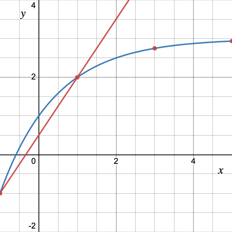
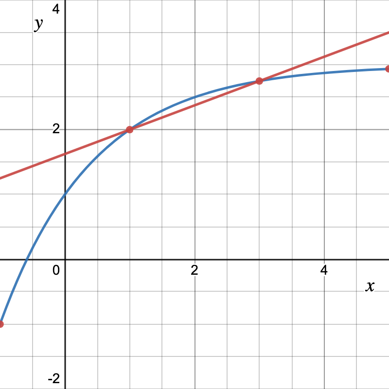
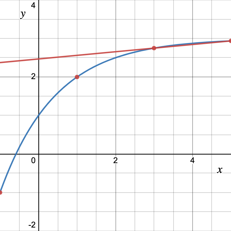
\(AV_{[-1,1]} = 1.5\text{,}\) \(AV_{[1,3]} \approx 0.375\text{,}\) and \(AV_{[3,5]} \approx 0.094\text{.}\) On \([-1,5]\text{,}\) the function \(h\) is increasing but at a decreasing rate.


1.4 Linear Functions
1.4.2 Properties of linear functions


1.4.3 Interpreting linear functions in context


Activity 1.4.3.

1.4.3.b
Answer.
The slope has units of \(\frac{\text{m}^2}{\text{year}}\text{,}\) or square meters per year, and represents how much the ice cover is changing each year. The \(A\)-intercept has units \(\text{m}^2\) and represents the amount of ice cover in the year \(2000\text{.}\)
1.4.3.c
Answer.
\(f(17) \approx 989\) m\(^2\text{.}\) This is the predicted area of the ice cover in the year \(2017\text{.}\)
1.4.3.d
Answer.
\(t \approx 34.5\text{,}\) which corresponds to the middle of the year \(2034\text{.}\)
1.4.3.e
Answer.
A reasonable domain is \(0 \le t \le 34.5\text{,}\) and the corresponding range is \(0 \le A \le 1951\text{.}\)


Activity 1.4.4.

1.4.4.b
Answer.
The slope is \(-465\text{.}\) This means the town’s population decreases by \(465\) people each year.
1.4.4.c
Answer.
\(p(t) = \frac{32\pi}{3} - 1.2t\text{.}\) A reasonable domain is \([0, 27.9]\text{.}\)
1.4.4.e
Answer.
\(C=L(t) = 15800 - 1120t\text{.}\) A reasonable domain is \([0, 14.1]\text{.}\) The slope is \(-1120\text{,}\) meaning the car loses \(\$1120\) in value each year.

1.5 Quadratic Functions
1.5.2 Properties of Quadratic Functions


Activity 1.5.2.

1.5.2.a
Answer.
If \(a > 0\) the parabola opens upward; if \(a < 0\) it opens downward. The larger \(|a|\) is, the narrower the parabola; the closer \(|a|\) is to zero, the wider the parabola.
1.5.2.b
Answer.
With \(a = 1\) and \(c = 0\text{,}\) changing \(b\) shifts the vertex diagonally: making \(b > 0\) moves the vertex left and down, while making \(b < 0\) moves it right and down.
1.5.2.c
Answer.
With \(a = 1\) and \(b = 0\text{,}\) changing \(c\) moves the vertex straight up or down along the \(y\)-axis.
1.5.2.d
Answer.
The parameter \(c\) seems to have the simplest effect while \(b\) seems to have the most complicated effect.


Activity 1.5.3.

1.5.3.d
Answer.
Two, because the vertex \((-1,9)\) is above the \(x\)-axis and the parabola opens downward. \(x=-1 \pm \sqrt{3}\)

1.5.3 Modeling falling objects


Activity 1.5.4.

1.5.4.e
Answer.
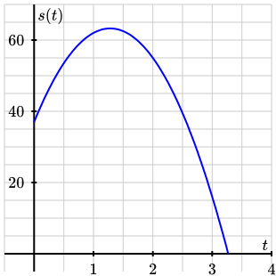
\(t = \frac{41}{32} \approx 1.28\) seconds; \(s\left(\frac{41}{32}\right) = \frac{4049}{64} \approx 63.3\) feet
1.5.4.f
Answer.
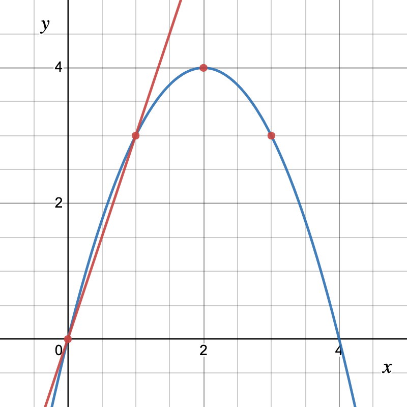
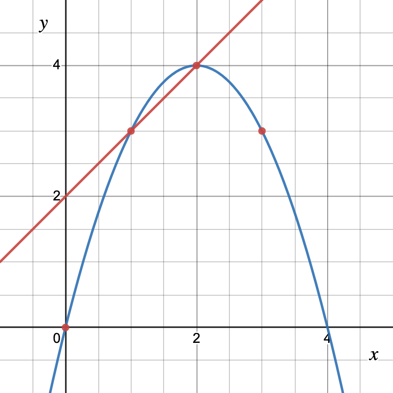
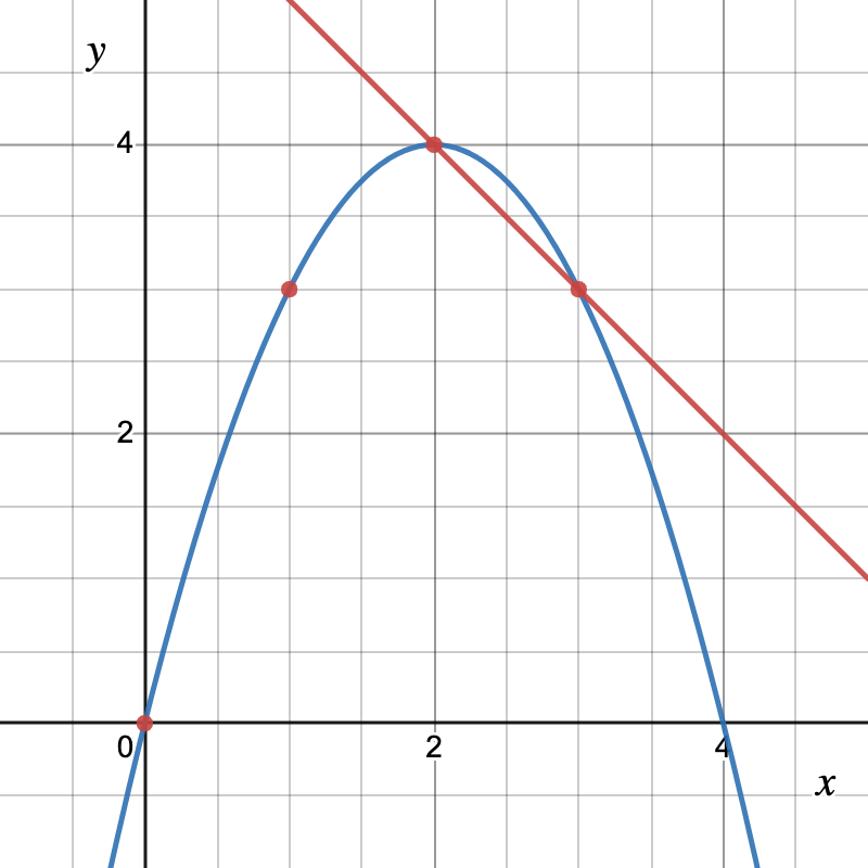
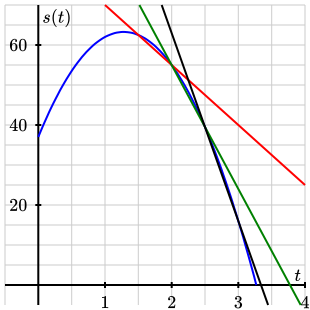
\(AV_{[1.5,2]} = -15 \text{ ft/s}, AV_{[2,2.5]} = -31 \text{ ft/s}, AV_{[2.5,3]} = -47 \text{ ft/s}\text{.}\) Between \(t=1.5\) and \(t=2\text{,}\) the water balloon is falling at an average rate of \(15\) feet per second; similarly for the other intervals. The balloon is falling faster and faster as it descends.
described in detail following the image
A graph of \(s(t)\) along with the lines representing the average rates of change on \([1.5,2]\text{,}\) \([2,2.5]\text{,}\) and \([2.5,3]\text{.}\)

1.6 Composite Functions
1.6.2 Composing two functions


Activity 1.6.2.

1.6.3 Composing functions in context


Activity 1.6.3.

1.6.3.b
Answer.
The function \(H\) converts the number of cricket chirps per minute directly into a temperature in degrees Celsius.
1.6.3.c
Answer.
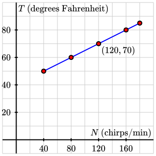
described in detail following the image
Plot of \(D(N)\) with horizontal axis labeled \(N\) (chirps per minute) and vertical axis in degrees Fahrenheit.
The graph is a line segment from \((40,50)\) to \((180,85)\text{,}\) also going through the points \((80, 60)\text{,}\) \((120, 70)\text{,}\) and \((160, 80)\text{.}\)
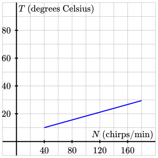
described in detail following the image
Plot of the function \(H(N)\) with horizontal axis labeled \(N\) (chirps per minute) and vertical axis labeled \(T\) (degrees Celsius).
The graph is a line segment from \((40,10)\) to \((180, \frac{265}{9})\text{.}\)
1.6.3.d
Answer.
The domain of \(H\) is \([40, 180]\) and the range is approximately \([10, 29.4]\text{.}\)

1.6.4 Function composition and average rate of change


1.7 Inverse Functions
1.7.2 When a function has an inverse function


1.7.3 Determining whether a function has an inverse function


Activity 1.7.3.

1.7.3.b
Answer.
The function \(g\) does have an inverse. For example, \(g^{-1}(4) = 0\) and \(g^{-1}(0) = 1\text{.}\)
1.7.3.c
Answer.
The function \(p\) does have an inverse. For example, \(p^{-1}(7) = 0\) and \(p^{-1}(4) = 5\text{.}\)
1.7.3.e
Answer.
The function \(r\) has an inverse, for example \(r^{-1}(2) = -1\) and \(r^{-1}(0) = 0\text{.}\) The function \(s\) does not have an inverse.

1.7.4 Properties of an inverse function


Activity 1.7.4.

1.7.4.a
Answer.
\(g(3) = 1.8\) cm/hr. At \(t = 3\) hours into the storm, the rain is falling at a rate of \(1.8\) centimeters per hour.
1.7.4.b
Answer.
\(AV_{[3,5]} = -\frac{4}{35}\) \(\text{cm/hr}^2\text{.}\) This means that between hours \(3\) and \(5\text{,}\) the rate of rainfall decreased on average by about \(0.114\) cm/hr per hour. We expect the rainfall rate to continue decreasing.
1.7.4.c
Answer.
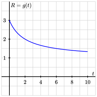
described in detail following the image
Graph of \(R=g(t)\text{,}\) which goes through \((0,3)\) and decreases curving upward until stopping at \((10,\frac{4}{3})\text{.}\)
The range of \(g\) on \([0,10]\) is \(\left[\frac{4}{3}, 3\right]\text{.}\) The function \(g\) has an inverse because it is strictly decreasing and passes the horizontal line test.
1.7.4.d
Answer.
\(g^{-1}\!\left(\frac{9}{5}\right) = 3\text{.}\) The rainfall rate equals \(1.8\) cm/hr at exactly \(3\) hours into the storm.
1.7.4.e
Answer.
No. Setting \(g(t) = 1\) gives \(\frac{4}{t+2} + 1 = 1\text{,}\) but \(\frac{4}{t+2} \gt 0\) for all \(t\) in \([0,10]\text{,}\) so there is no solution.

1.8 Transformations of Functions
1.8.2 Translations of Functions


Activity 1.8.2.

1.8.2.a
Answer.
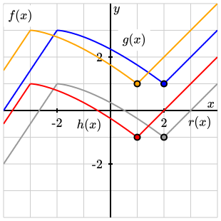
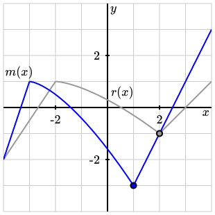
The function \(g(x)\) shifts \(r\) up 2 units, while the function \(h(x)\) shifts \(r\) left 1 unit, and the function \(f(x)\) shifts \(r\) both up 2 and left 1.
described in detail following the image
A parent function \(r(x)\) along with three transformations: \(h(x)\) which shifts to the left 1 unit, \(g(x)\) which shifts up 2 units, and \(f(x)\) which shifts both left 1 unit and up 2 units.
1.8.2.b
Answer.
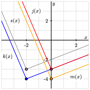
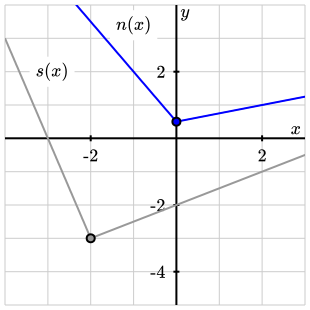
The function \(k(x)\) shifts \(s\) down 1 unit, while the function \(j(x)\) shifts \(s\) right 2 units, and the function \(m(x)\) shifts \(s\) both down 1 and right 2.
described in detail following the image
A parent function \(s(x)\) along with three transformations: \(j(x)\) which shifts to the right 2 units, \(k(x)\) which shifts down 1 units, and \(m(x)\) which shifts both right 2 units and down 1 unit.
1.8.2.c
Answer.
The function \(p(x)=x^2 + 6x + 5\text{,}\) and is the result of translating \(q(x)\) three units to the left and four units down.

1.8.3 Vertical stretches and reflections


Activity 1.8.3.

1.8.3.a
Answer.
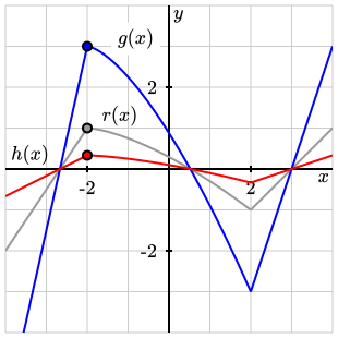
The graph of \(g(x) = 3r(x)\) is a vertical stretch of \(r\) by a factor of \(3\) while the graph of \(h(x) = \frac{1}{3}r(x)\) is a vertical compression of \(r\) by a factor of \(\frac{1}{3}\text{.}\)
described in detail following the image
A parent function \(r(x)\) along with two transformations: \(g(x)\) which stretches vertical heights by a factor of 3, and \(h(x)\) which vertically compresses vertical heights by a factor of 1/3.
1.8.3.b
Answer.
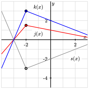
The graph of \(k(x) = -s(x)\) is a reflection of \(s\) across the \(x\)-axis, while the graph of \(j(x) = -\frac{1}{2}s(x)\) is a vertical compression by \(\frac{1}{2}\) combined with a reflection across the \(x\)-axis.
described in detail following the image
A parent function \(s(x)\) along with two transformations: \(k(x)\) which reflects heights over the \(x\)-axis and \(j(x)\) which reflects and vertically compresses vertical heights by a factor of 1/2.
1.8.3.c
Answer.
described in detail following the image
A parent function \(r(x)\) along with a transformation \(m(x)\) which shifts left 1 unit, stretches vertical heights by a factor of 2, and shifts down by 1 unit.
described in detail following the image
A parent function \(s(x)\) along with a transformation \(n(x)\) which shifts right 2 units, compresses vertical heights by a factor of 1/2, and shifts up by 2 units.
1.8.3.d
Answer.
The function \(m(x) = 2r(x+1) - 1\) results from three elementary transformations of \(r\text{:}\) a horizontal shift left 1 unit (replacing \(x\) with \(x+1\)), a vertical stretch by a factor of 2 (multiplying by 2), and a vertical shift down 1 unit (subtracting 1). The vertical stretch and the horizontal shift may be applied in either order, but both must be applied before the vertical shift.
1.8.4 Combining shifts and stretches: why order sometimes matters


Activity 1.8.4.

1.8.4.a
Answer.
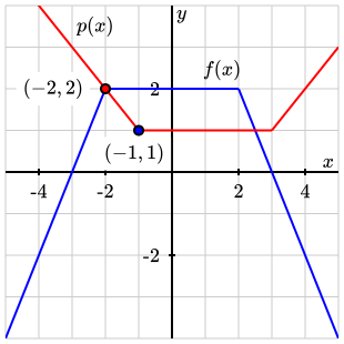
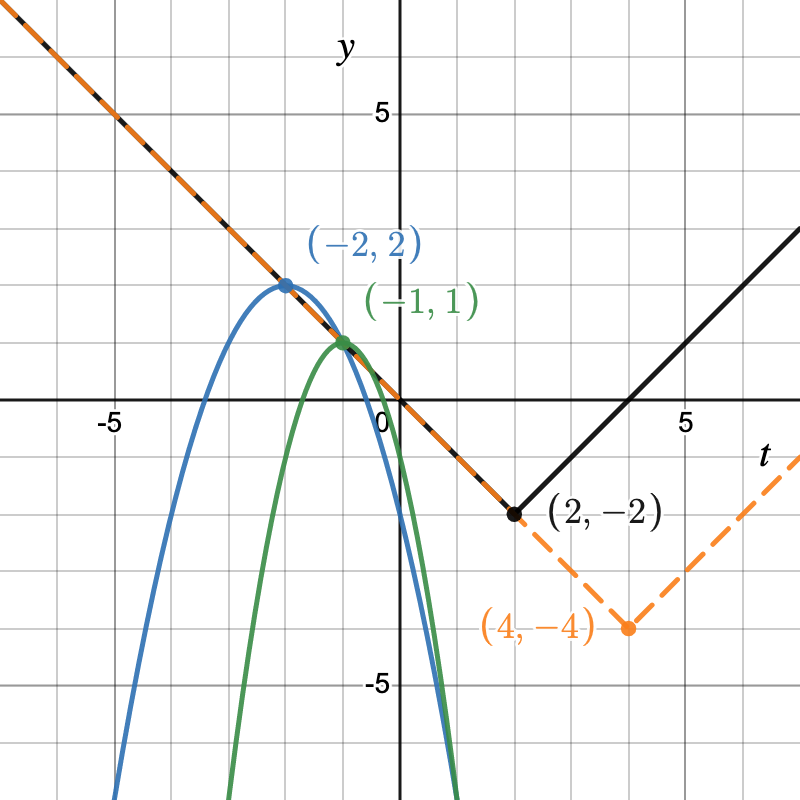
Shift right 1 unit, then compress vertically by a factor of \(\frac{1}{2}\text{,}\) then reflect across the \(x\)-axis, and lastly shift up 2 units. The point \((-2, 2)\) on \(f\) moves to \((-1, 1)\) on \(p\text{.}\)
described in detail following the image
Graph of the piecewise linear function \(f(x)\text{,}\) along with a transformation of \(f\text{.}\)
The function \(p(x)\) is also piecewise linear, but has been flipped upside-down, shrunk vertically so that the slopes of each line are half what they are in \(g\text{,}\) and shifted to the right. The point \((-1,1)\) is marked on the graph of \(p\text{.}\)
1.8.4.b
Answer.
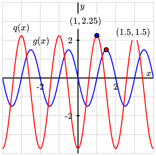
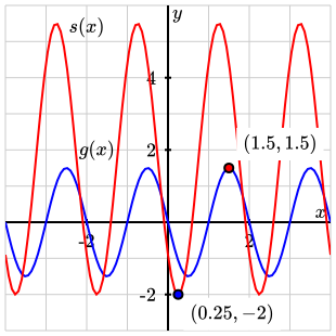
Shift left \(0.5\) units, then stretch vertically by a factor of 2, and lastly shift down \(0.75\) units. The point \((1.5, 1.5)\) on \(g\) moves to \((1, 2.25)\) on \(q\text{.}\)
described in detail following the image
Graph of the function \(g(x)\text{,}\) along with a transformation of \(g\text{.}\)
The function \(g\) is going up and down repeatedly, hitting peaks of \(1.5\) and valleys of \(-1.5\text{.}\) The point \((1.5,1.5)\) is marked on the graph of \(g\text{.}\)
The function \(q(x)\) is also going up and down repeatedly, but reaches higher peaks and valleys and has been shifted horizontally. The point \((1,2.25)\) is marked on the graph of \(q\text{.}\)
1.8.4.c
Answer.
Both shift \(f\) right 1 unit and apply a vertical compression and reflection by \(-\frac{1}{2}\text{,}\) but \(p\) then shifts the result up 2 units while \(r\) shifts it down 2 units.
1.8.4.d
Answer.
\(s(x) = -2.5\,g(x+1.25) + 1.75.\)
described in detail following the image
Graph of a function \(g(x)\) which is going up and down repeatedly, hitting peaks of \(1.5\) and valleys of \(-1.5\text{.}\) The point \((1.5,1.5)\) is marked on the graph.

1.9 Combining Functions
1.9.2 Arithmetic with functions


Activity 1.9.2.

1.9.2.f
Answer.
\((f-g)(x) = 0\) at one value between \(x=0\) and \(x=1\text{.}\) Using algebraic formulas for the functions, \(x = \dfrac{\sqrt{7}-1}{2}\)

1.9.3 Combining functions in context


Activity 1.9.3.

1.9.3.a
Answer.
At a speed of 60 miles per hour, the car consumes 0.04 gallons of fuel for each mile traveled.
1.9.3.b
Answer.
\(g(60) = 25\) miles per gallon. The function \(g\) measures the car’s fuel economy in miles per gallon at a given input speed.
1.9.3.c
Answer.
\(h(60) = 2.4\) gallons per hour. The function \(h\) measures the rate at which the car consumes fuel (in gallons per hour) at a given speed.
1.9.3.d
Answer.
All three convey information about the fuel consumption at \(60\) mph, but with different units and perspectives.
1.9.3.e
Answer.
\(AV_{[60,70]} = 0.0005 \ \frac{\text{gal/mi}}{\text{mph}}.\) This measures how much the car’s fuel consumption rate (in gallons per mile) increases per additional mile per hour of speed.

1.9.4 Piecewise functions


Activity 1.9.4.

1.9.4.a
Answer.
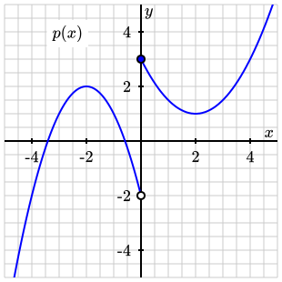
\(p(-4) = -2\text{;}\) \(p(-2) = 2\text{;}\) \(p(0) = 3\text{;}\) \(p(2) = 1\text{;}\) \(p(4) = 3\text{.}\)
1.9.4.b
Answer.
The parabola that is valid for \(x \lt 0\) has vertex \((-2, 2)\text{.}\) The parabola that is valid for \(x \ge 0\) has vertex \((2, 1)\text{.}\)
1.9.4.c
Answer.
\(p(x)=0\) when \(x = -2 + \sqrt{2} \approx -0.586\) and \(x = -2 - \sqrt{2} \approx -3.414\text{.}\) The \(y\)-intercept is \(p(0) = 3\text{.}\)
1.9.4.d
Answer.
described in detail following the image
A piecewise function \(p(x)\text{.}\) The first piece is an downward-opening parabola with vertex \((-2,2)\) ending in an open circle at \((0,-2)\text{,}\) while the second piece is an upward-opening parabola starting at a closed circle at \((0,3)\) with vertex \((2,1)\text{.}\)
1.9.4.e
Answer.
\begin{equation*} f(x) = \begin{cases} 3 - \frac{1}{2}(x+1), \amp -2.5 \lt x \le -1 \\ 4 + \frac{3}{2}(x-1), \amp -1 \lt x \le 1 \\ 1 - \frac{3}{4}(x-1), \amp 1 \lt x \lt 3.5, \ x \ne 2 \end{cases} \end{equation*}

2 Circular Functions
2.1 Traversing Circles
2.1.2 Circular Functions


Activity 2.1.2.

2.1.2.b
Answer.
The \(y\)-coordinate of \(P_2\) is \(2 - \frac{4}{\pi} = \frac{2(\pi - 2)}{\pi}\text{.}\) The \(y\)-coordinate of \(P_4\) is \(2\text{.}\)
2.1.2.c
Answer.
\(d\) \(0\) \(1\) \(2\) \(3\) \(4\) \(5\) \(6\) \(7\) \(8\)
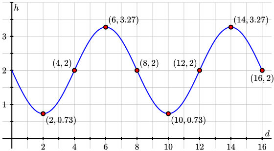
\(h\) \(2\) \(1.10\) \(0.73\) \(1.10\) \(2\) \(2.90\) \(3.27\) \(2.90\) \(2\)
\(d\) \(9\) \(10\) \(11\) \(12\) \(13\) \(14\) \(15\) \(16\)
\(h\) \(1.10\) \(0.73\) \(1.10\) \(2\) \(2.90\) \(3.27\) \(2.90\) \(2\)
2.1.2.d
Answer.
described in detail following the image
Graph of \(h\) versus \(d\) with points marked at \(d=2,4,6,8,10,12,14\) and \(16\text{.}\)
2.1.2.e
Answer.
This graph is shifted up, shifted to the right, and is compressed horizontally compared to the textbook figure.

2.1.3 Properties of Circular Functions


Activity 2.1.3.

2.1.3.a
Answer.
The period of the motion is \(p = 4\) seconds. The midline is \(y = 8\) inches. The amplitude is \(a = 5\) inches.
2.1.3.b
Answer.
The greatest displacement of the weight is \(13\) inches. The least displacement is \(3\) inches. The range of \(f\) is \([3, 13]\text{.}\)
2.1.3.c
Answer.
\(AV_{[4,4.25]}= -4.772\) inches per second on the interval \([4,4.25]\text{.}\)
\(AV_{[4.75,5]} = -1.524\) inches per second on the interval \([4.75,5]\text{.}\)
The average rate of change of this function represents the speed of the weight. Taken together, these two values indicate that the weight is moving more slowly on the interval \([4.75,5]\) than on the interval \([4,4.25]\text{,}\) but that the weight is moving in the same direction on each of these intervals.

2.1.4 The average rate of change of a circular function


Activity 2.1.4.

2.1.4.a
Answer.
  • \(AV_{[2,2.25]} \approx 7.652\) inches/sec
  • \(AV_{[2.25,2.5]} \approx 6.492\) inches/sec
  • \(AV_{[2.5,2.75]} \approx 4.332\) inches/sec
  • \(AV_{[2.75,3]} \approx 1.524\) inches/sec
The weight is always moving in the same direction (away from the wall) on the interval \([2,3]\text{,}\) but is slowing down.
2.1.4.b
Answer.
The weight slows down as it reaches the farthest distance away from the midline and speeds up back toward the center. The greatest (steepest) negative rates of change occur near the midline where the function is decreasing, in intervals such as \([0, 0.25]\text{,}\) \([3.75, 4.00]\text{,}\) and \([4.00, 4.25]\text{.}\)
2.1.4.c
Answer.
Examples of longest such intervals are \([3,5]\text{,}\) \([7,9]\text{,}\) and \([11,13]\text{.}\)
2.1.4.d
Answer.
The intervals on which \(f\) is concave up include \([0,2]\text{,}\) \([4,6]\text{,}\) \([8,10]\text{,}\) and \([12,14]\text{.}\)
2.1.4.f
Answer.
At the highest and lowest points, the function has the smallest rates of change. Near the midline, the function has its greatest rates of change.

2.2 The Unit Circle
2.2.2 Radians and degrees


2.2.3 Special points on the unit circle


Activity 2.2.3.

2.2.3.b
Answer.
The resulting shape forms an equilateral triangle where all three interior angles are \(60^\circ\) and all sides have the same length, 1 unit. Thus, \(y = \frac{1}{2}\) and by the Pythagorean theorem, \(x = \frac{\sqrt{3}}{2}\text{.}\)
2.2.3.d
Answer.
The coordinates of the point at \(\theta = \frac{\pi}{6}\) on the unit circle are \(\left( \frac{\sqrt{3}}{2}, \frac{1}{2} \right)\text{.}\) The coordinates at \(\theta = \frac{\pi}{4}\) are \(\left( \frac{\sqrt{2}}{2}, \frac{\sqrt{2}}{2} \right)\text{.}\) The coordinates at \(\theta = \frac{\pi}{3}\) are \(\left( \frac{1}{2}, \frac{\sqrt{3}}{2} \right)\text{.}\)

2.2.4 Special points and arc length in non-unit circles


2.3 The Sine and Cosine Functions
2.3.3 The definition of the cosine function


Activity 2.3.2.

2.3.2.a
Answer.
\(\cos\left(\frac{\pi}{6}\right) = \frac{\sqrt{3}}{2}\text{;}\) \(\cos\left(\frac{5\pi}{6}\right) = -\frac{\sqrt{3}}{2}\text{;}\) \(\cos\left(-\frac{\pi}{3}\right) = \frac{1}{2}\text{.}\)
2.3.2.b
Answer.
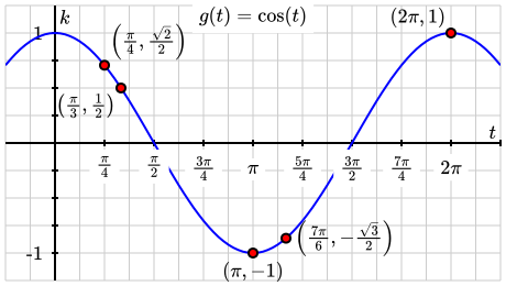
\(t\) \(0\) \(\frac{\pi}{6}\) \(\frac{\pi}{4}\) \(\frac{\pi}{3}\) \(\frac{\pi}{2}\) \(\frac{2\pi}{3}\) \(\frac{3\pi}{4}\) \(\frac{5\pi}{6}\) \(\pi\)
\(k\) \(1\) \(\frac{\sqrt{3}}{2}\) \(\frac{\sqrt{2}}{2}\) \(\frac{1}{2}\) \(0\) \(-\frac{1}{2}\) \(-\frac{\sqrt{2}}{2}\) \(-\frac{\sqrt{3}}{2}\) \(-1\)
\(t\) \(\pi\) \(\frac{7\pi}{6}\) \(\frac{5\pi}{4}\) \(\frac{4\pi}{3}\) \(\frac{3\pi}{2}\) \(\frac{5\pi}{3}\) \(\frac{7\pi}{4}\) \(\frac{11\pi}{6}\) \(2\pi\)
\(k\) \(-1\) \(-\frac{\sqrt{3}}{2}\) \(-\frac{\sqrt{2}}{2}\) \(-\frac{1}{2}\) \(0\) \(\frac{1}{2}\) \(\frac{\sqrt{2}}{2}\) \(\frac{\sqrt{3}}{2}\) \(1\)
2.3.2.d
Answer.
\(\cos\left(\frac{11\pi}{4}\right) = \cos\left(\frac{3\pi}{4}\right) = -\frac{\sqrt{2}}{2}\text{;}\) and \(\cos\left(\frac{14\pi}{3}\right) = \cos\left(\frac{2\pi}{3}\right) = -\frac{1}{2}\text{.}\)
2.3.2.e
Answer.
\(\cos(t) = -\frac{\sqrt{3}}{2}\) for \(t = \frac{5\pi}{6},\ \frac{7\pi}{6},\ \frac{17\pi}{6},\ \frac{19\pi}{6}\text{.}\)
2.3.2.f
Answer.
The graphs of \(k = \cos(t)\) and \(h = \sin(t)\) are the same after a horizontal shift of \(\frac{\pi}{2}\text{.}\)

2.3.4 Properties of the sine and cosine functions


Activity 2.3.3.

2.3.3.f
Answer.
The most rapid average rates of change on both graphs occur near the zero crossing points (where the function crosses the midline).

2.3.5 Using computing technology


Activity 2.3.4.

2.3.4.f
Answer.
\begin{equation*} AV_{[0.1,0.2]} \approx 0.98836 \end{equation*}
\begin{equation*} AV_{[0.8,0.9]} \approx 0.65971 \end{equation*}
2.3.4.g
Answer.
\begin{equation*} AV_{[0.1,0.2]} \approx -0.14938 \end{equation*}
\begin{equation*} AV_{[0.8,0.9]} \approx -0.75097 \end{equation*}

2.4 Sinusoidal Functions
2.4.2 Shifts and vertical stretches of the sine and cosine functions


Activity 2.4.2.

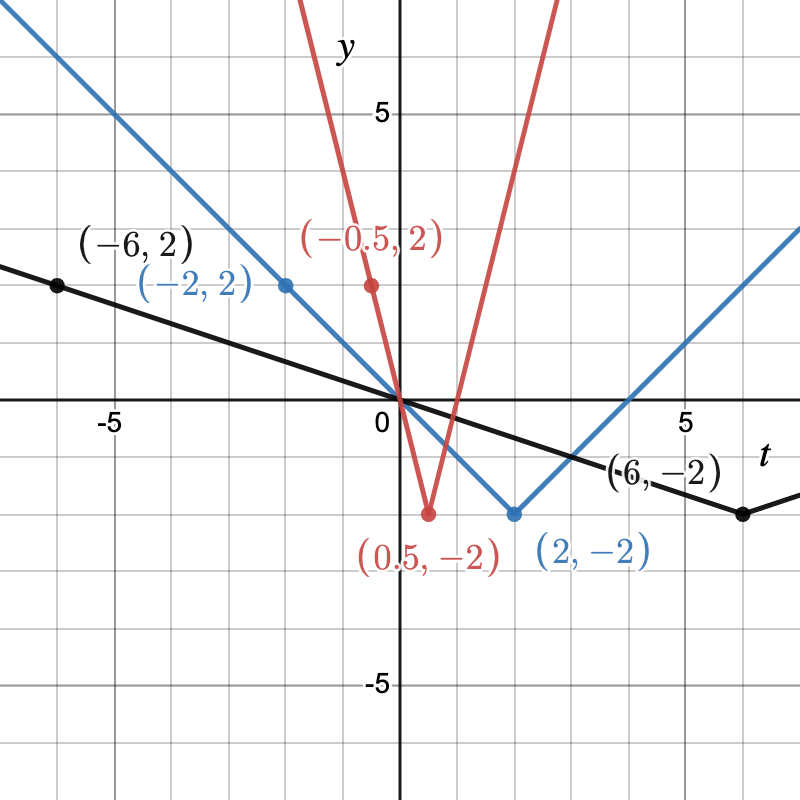
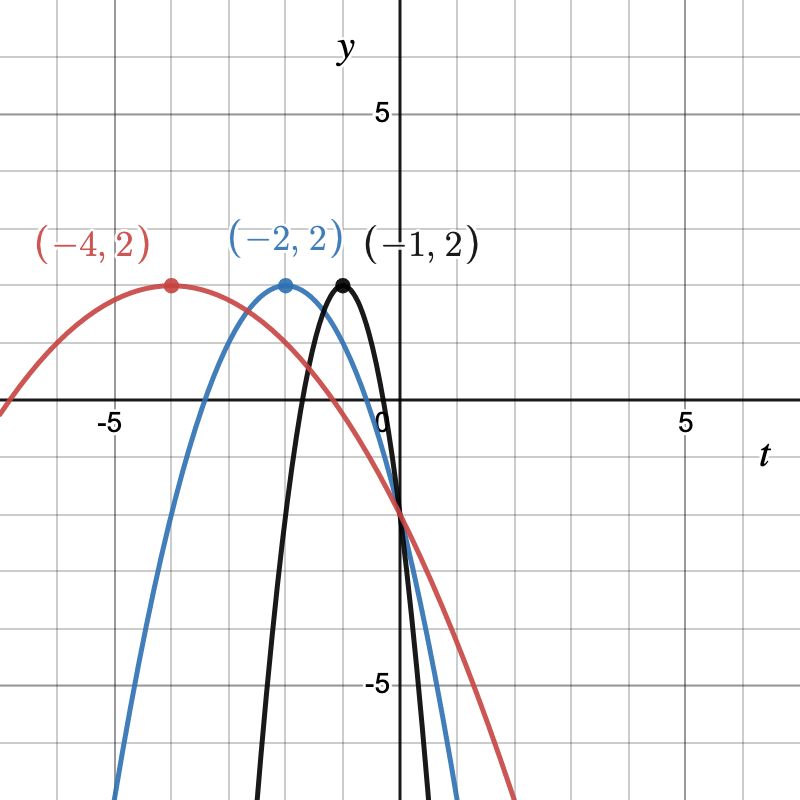
Answer.
One formula is \(d(t) = -2.5\sin(t) + 4.5\text{,}\) which has an anchor point with coordinates \((0, 4.5)\text{.}\) Another formula with the same anchor point is \(d(t) = 2.5\cos\left(t + \frac{\pi}{2}\right) + 4.5\text{.}\)

2.4.3 Horizontal scaling


Activity 2.4.3.

2.4.3.a
Answer.
The function \(h(t) = f\!\left(\frac{1}{3}t\right)\) represents a horizontal scaling of \(f\) by a factor of 3 (stretching). The function \(j(t) = f(4t)\) represents a horizontal scaling by a factor of \(\frac{1}{4}\) (compression).
described in detail following the image
Graphs of two horizontal scaling functions of \(f(x)\)
2.4.3.b
Answer.
The function \(k(t) = g(2t)\) represents a horizontal scaling of \(g\) by a factor of \(\frac{1}{2}\) (compression). The function \(m(t) = g\!\left(\frac{1}{2}t\right)\) represents a horizontal scaling by a factor of 2 (stretching).
described in detail following the image
Graphs of two horizontal scaling functions of \(g(x)\)
2.4.3.c
Answer.
The function \(r(t) = 2f\!\left(\frac{1}{2}t\right)\) applies both a horizontal scaling by a factor of 2 and a vertical scaling by a factor of 2. The function \(s(t) = \frac{1}{2}g(2t)\) applies both a horizontal scaling by a factor of \(\frac{1}{2}\) and a vertical scaling by a factor of \(\frac{1}{2}\text{.}\)
described in detail following the image
Graphs of transformations which scale both horizontally and vertically.
2.4.3.d
Answer.
The function \(r(t) = 2f\!\left(\frac{1}{2}t\right)\) is both a vertical and a horizontal scaling. The order does not matter

2.4.4 Circular functions with different periods


Activity 2.4.4.

2.4.4.a
Answer.
Period \(\frac{\pi}{5}\text{,}\) amplitude 1, midline \(y=2\text{,}\) range \([1,3]\text{,}\) no horizontal shift, anchor point \((0,2)\text{.}\)
2.4.4.b
Answer.
Period \(8\pi\text{,}\) amplitude 3 (with reflection), midline \(y=-4\text{,}\) range \([-7,-1]\text{,}\) no horizontal shift, anchor point \((0,-7)\text{.}\)
2.4.4.c
Answer.
Period 8, amplitude 2, midline \(y=5\text{,}\) range \([3,7]\text{,}\) no horizontal shift, anchor point \((0,5)\text{.}\)
2.4.4.d
Answer.
Period 4, amplitude 2, midline \(y=5\text{,}\) range \([3,7]\text{,}\) horizontal shift 3 units to the right, anchor point \((0,5)\text{.}\)
2.4.4.e
Answer.
Note that \(u(x) = -0.25\sin(3(x-2)) + 5\text{.}\) Period \(\frac{2\pi}{3}\text{,}\) amplitude \(0.25\text{,}\) midline \(y=5\text{,}\) range \([4.75,5.25]\text{,}\) horizontal shift 2 units to the right. The anchor point is at approximately \((0, 4.93)\text{,}\) since \(u(0) = -0.25\sin(-6)+5\) is not a convenient exact value.


Activity 2.4.5.

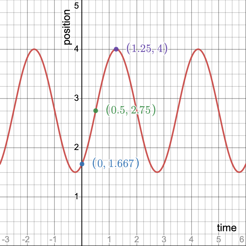
Answer.
The midline is \(c = \frac{1.5+4}{2} = 2.75\) feet, the amplitude is \(a = \frac{4-1.5}{2} = 1.25\) feet, the range is \([1.5,4]\text{,}\) and the anchor point is at approximately \((0, 1.67)\text{.}\) The formula is \(d(t) = 1.25\cos\!\left(\frac{2\pi}{3}(t - 1.25)\right) + 2.75 \text{.}\)
described in detail following the image
Graph of \(d(t)\)

3 Exponential and Logarithmic Functions
3.1 Exponential Growth and Decay
3.1.2 Exponential functions of form \(f(t) = ab^t\)


Activity 3.1.2.

3.1.2.d
Answer.
When \(b\) is less than \(1\text{,}\) the function is decreasing and concave up, approaching \(0\) as \(x\) gets larger and larger. When When \(b\) is greater than \(1\text{,}\) the function is increasing and concave up, approaching \(\infty\) as \(x\) gets larger and larger.
3.1.2.e
Answer.
When \(b\) is greater than \(1\text{,}\) the function describes positive growth (growing with time). When \(b\) is between \(0\) and \(1\text{,}\) the function describes negative growth (decreasing with time).
3.1.2.f
Answer.
We can tell that \(0 \lt b \lt 1\) while \(d \gt 1\text{.}\) Also, \(a \gt c\text{.}\)

3.1.3 Determining formulas for exponential functions


Activity 3.1.3.

3.1.3.a
Answer.
Exactly: \(b = \left( \dfrac{13}{25} \right)^{1/4}\text{,}\) \(a = 12500 \left( \dfrac{25}{13} \right)^{3/4} = 6500 \left( \dfrac{25}{13} \right)^{7/4}\text{.}\) In approximate form, \(V(t) \approx \$ 20413 \cdot (0.8492)^t\text{.}\)
3.1.3.b
Answer.
The purchase value of the car is approximately \(\$ 20413\text{,}\) and the car is worth less than \(\$ 1000\) after a little over \(18\) years.
3.1.3.c
Answer.
\(L(t) = 17000 - 1500t\text{,}\) and the car will be worth \(\$ 1000\) when \(t = \frac{32}{3} \approx 10.67\) years.
3.1.3.d
Answer.
The exponential model seems more realistic because new cars decrease in value faster rate at the beginning and more slowly as they get older.

3.1.4 Trends in the behavior of exponential functions


Activity 3.1.4.

3.1.4.c
Answer.
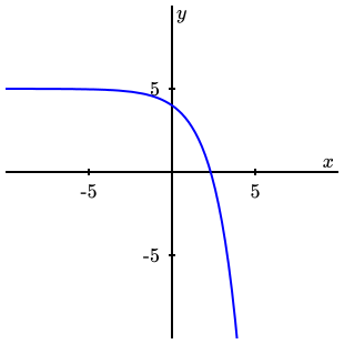
One option is a downward-opening parabola, such as \(-(x-2)^2+4\text{.}\)
described in detail following the image
A downward-opening parabola which has its peak at \(x=2\text{.}\)
3.1.4.d
Answer.
For example, \(s(x) = -\left(\frac{1}{2}\right)^x+5\text{.}\)
described in detail following the image
The function \(-\left(\frac{1}{2}\right)^x+5\text{,}\) which is increasing at a decreasing rate.
3.1.4.e
Answer.
For example, \(s(x) = -\left(\frac{1}{2}\right)^{-x}+5\text{.}\)
described in detail following the image
The function \(-\left(\frac{1}{2}\right)^{-x}+5\text{,}\) which is decreasing at a decreasing rate.

3.2 Modeling with exponential functions
3.2.3 The role of \(c\) in \(g(t) = ab^t + c\)


Activity 3.2.2.

3.2.2.a
Answer.
The function \(p(t) = ab^t+c = 4372(1.000235)^t + 92856\) has \(a \gt 0\) and \(b \gt 1\text{,}\) so \(p(t)\) is always increasing, always concave up, and increasing without bound and has been shifted vertically up by \(92856\text{.}\) The \(y\)-intercept is \(p(0) = 4372+92856= 97228\) and the range is \((92856, \infty)\text{.}\)
3.2.2.b
Answer.
The function \(q(t) = 27931(0.97231)^t + 549786\) is always decreasing, always concave up, and decreasing toward \(549786\text{.}\) The \(y\)-intercept is \(q(0) = 577717\) and the range is \((549786, \infty)\text{.}\)
3.2.2.c
Answer.
The function \(r(t) = -17398(0.85234)^t\) is always increasing, always concave down, and increasing toward \(0\text{.}\) The \(y\)-intercept is \(r(0) = -17398\) and the range is \((-\infty, 0)\text{.}\)
3.2.2.d
Answer.
The function \(s(t) = -17398(0.85234)^t + 19411\) is always increasing, always concave down, and increasing toward the value \(19411\text{.}\) The \(y\)-intercept is \(s(0) = 2013\) and the range is \((-\infty, 19411)\text{.}\)
3.2.2.e
Answer.
The function \(u(t) = -7522(1.03817)^t\) is always decreasing, always concave down, and decreasing without bound. The \(y\)-intercept is \(u(0) = -7522\) and the range is \((-\infty, 0)\text{.}\)
3.2.2.f
Answer.
The function \(v(t) = -7522(1.03817)^t + 6731\) is always decreasing, always concave down, and decreasing without bound. The \(y\)-intercept is \(v(0) = -791\) and the range is \((-\infty, 6731)\text{.}\)

3.2.4 Modeling temperature data


Activity 3.2.3.

3.2.3.a
Answer.
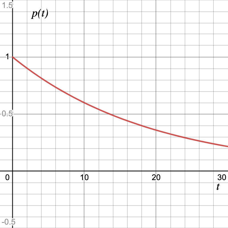
The graph of \(p(t) = (0.95)^t\) is always decreasing, always concave up, and decreasing toward zero.
described in detail following the image
graph of \(p(t) = (0.95)^t\)
3.2.3.b
Answer.
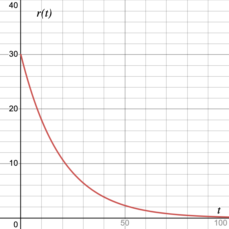
The function \(r(t) = 30(0.95)^t\) is similar to \(p(t)\) but stretched vertically by a factor of \(30\text{.}\) It is always decreasing, always concave up, and decreasing toward zero.
described in detail following the image
graph of \(r(t) = 30 (0.95)^t\)
3.2.3.c
Answer.
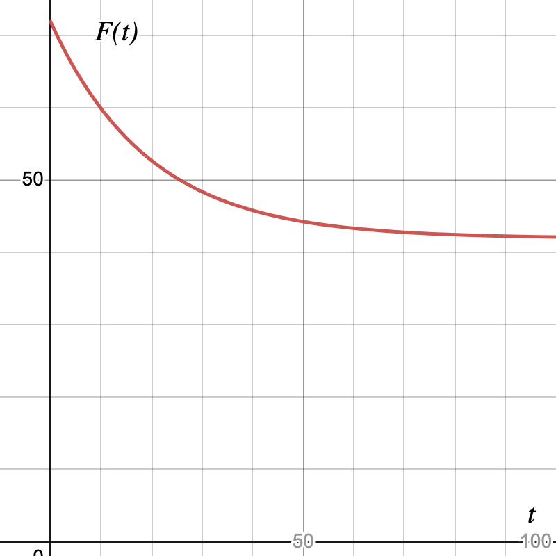
Since \(F(t) = 42 + 30(0.95)^t\) has a vertical shift of \(42\) up, it remains always decreasing, always concave up, but decreasing toward \(42\text{.}\)
described in detail following the image
graph of \(F(t) = 42+ 30 (0.95)^t\)
3.2.3.d
Answer.
The temperature of the refrigerator is \(42\text{.}\) The room temperature of the surroundings outside the refrigerator is \(72\text{.}\)
3.2.3.e
Answer.
\begin{equation*} AV_{[10,20]} & \approx -0.721 \text{ degrees per minute} \\ AV_{[20,30]} & \approx -0.432 \text{ degrees per minute} \\ AV_{[30,40]} & \approx -0.258 \text{ degrees per minute} \end{equation*}
The average rate of change is always negative and is decreasing in magnitude as \(t\) increases. This is consistent with a function that is always decreasing and always concave up. In context, the soda is cooling more and more slowly as time goes on.


Activity 3.2.4.

3.2.4.b
Answer.
The expression \((0.98)^t\) approaches zero as \(t\) gets large, so \(F(t) \to a\text{,}\) and therefore \(a = 212^\circ\text{.}\)
3.2.4.d
Answer.
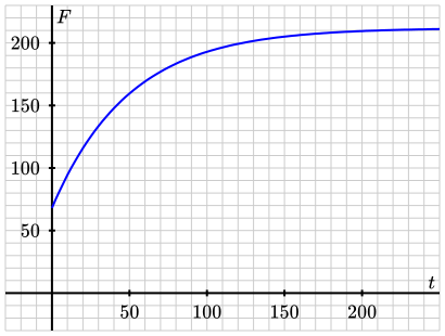
The function \(F(t) = 212 - 144(0.98)^t\) is shown below. The potato reaches \(180\) degrees after about \(75\) minutes of baking in the \(350\) degree oven.
described in detail following the image
Graph of \(F(t)=212-144(0.98)^t\text{.}\)
3.2.4.e
Answer.
We can view \(F(t) = a - b(0.98)^t\) as a transformation of the parent function \(f(t) = (0.98)^t\) by first stretching \(f\) vertically by a factor of \(b\text{,}\) then reflecting over the \(t\)-axis, and finally shifting vertically up by \(a\) units.

3.3 The special number \(e\)
3.3.2 The natural base \(e\)


Activity 3.3.2.

3.3.2.a
Answer.
\(A(0.5)\) gives the average rate of change of \(f(t) = e^t\) on the interval \([1, 1.5]\text{,}\) which is the slope of the line between the points \((1,f(1))\) and \((1.5,f(1.5))\text{.}\)
3.3.2.b
Answer.
\(h\) \(A(h)\)
\(0.01\) \(2.7319\)
\(0.001\) \(2.7196\)
\(0.0001\) \(2.7184\)
\(-0.0001\) \(2.7181\)
\(-0.001\) \(2.7169\)
\(-0.01\) \(2.7047\)
3.3.2.c
Answer.
As \(h\) gets smaller and smaller, the value of \(A(h)\) approaches the value of \(e\text{.}\)
3.3.2.d
Answer.
The statement makes sense because the rate of change on small intervals near \(t = 1\) is close to the value of \(e^1 = e\text{.}\)
3.3.2.e
Answer.
The value of \(A(h)\) near \(h = 0\) appears to be the same as the value of \(f(2) = e^2\text{.}\)

3.3.3 Why any exponential function can be written in terms of \(e\)


3.4 What a logarithm is
3.4.2 The base-\(10\) logarithm


Activity 3.4.2.

3.4.3 The natural logarithm


Activity 3.4.3.

3.4.3.a
Answer.
The domain of \(E(t) = e^t\) is all real numbers, and its range is all positive real numbers.
3.4.3.b
Answer.
The domain of \(N(y) = \ln(y)\) is all positive real numbers, and its range is all real numbers.
3.4.3.e
Answer.
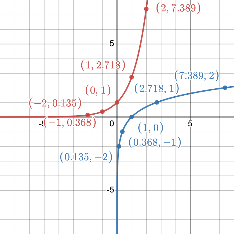
\(t\) \(-2\) \(-1\) \(0\) \(1\) \(2\)
\(E(t) = e^t\) (exact) \(e^{-2}\) \(e^{-1}\) \(1\) \(e\) \(e^2\)
\(E(t) = e^t\) (approx.) \(0.135\) \(0.368\) \(1\) \(2.718\) \(7.39\)
\(y\) \(e^{-2}\) \(e^{-1}\) \(1\) \(e^1\) \(e^2\)
\(N(y) = \ln(y)\) \(-2\) \(-1\) \(0\) \(1\) \(2\)
described in detail following the image
graphs of \(e^t\) and \(\ln(t)\) with points from the tables labeled on the graphs

3.4.4 \(f(t) = b^t\) revisited


Activity 3.4.4.

3.4.4.g
Answer.
There is no solution because the equation gives \(e^{2t} = -\frac{2}{3}\text{,}\) and there is no exponent for which \(e\) raised to that power is negative.

3.5 Properties and applications of logarithmic functions
3.5.2 Key properties of logarithms


Activity 3.5.2.

3.5.3 The graph of the natural logarithm


Activity 3.5.3.

3.5.3.a
Answer.
Both \(f(t) = 1 - e^{-(t-1)}\) and \(g(t) = \ln(t)\) are always increasing and concave down, and both have a \(t\)-intercept at \(t = 1\text{.}\) The domain of \(f\) is all real numbers, while the domain of \(g\) is all positive real numbers. The range of \(f\) is the interval \((-\infty, 1)\text{,}\) while the range of \(g\) is all real numbers. The \(y\)-intercept of \(f\) is \(f(0) = 1 - e \approx -1.718\text{,}\) while \(g\) has no \(y\)-intercept since \(t = 0\) is not in its domain. As \(t \to \infty\text{,}\) \(f(t) \to 1\) (bounded), while \(g(t) \to \infty\) (unbounded).
3.5.3.b
Answer.
The function \(h(t) = a - be^{-k(t-c)}\) is a transformation of \(E(t) = e^t\) in which \(E(t)\) is reflected over the horizontal axis and vertically stretched by a factor of \(b\text{,}\) horizontally compressed by a factor of \(k\) (with a horizontal reflection), shifted horizontally to the right by \(c\) units, and shifted vertically up by \(a\) units.
3.5.3.c
Answer.
The function \(r(t) = a + b\ln(t - c)\) is a transformation of \(L(t) = \ln(t)\) that is vertically stretched by a factor of \(b\text{,}\) shifted horizontally to the right by \(c\) units, and shifted vertically up by \(a\) units.
3.5.3.d
Answer.
Experimenting with Desmos, the exponential model \(q(t) = m + ne^{-rt}\) provides a good fit to the data; for instance, \(q(t) = 20.3 - 20.8e^{-0.35t}\) fits well. A logarithmic model is not as effective because the data levels off at a horizontal asymptote, which is consistent with an exponential model of the form \(a + be^{-kt}\) but not with a logarithmic model whose values grow without bound.

3.5.4 Putting logarithms to work


3.6 Modeling temperature and population
3.6.2 Newton’s Law of Cooling revisited


Activity 3.6.2.

3.6.2.a
Answer.
Since the soda cools toward the refrigerator temperature in the long run, and \(e^{-kt} \to 0\) as \(t \to \infty\text{,}\) we have \(c = 37.7\text{.}\) At \(t = 0\text{,}\) \(F(0) = a + c = a + 37.7 = 72.3\text{,}\) so \(a = 34.6\text{.}\)
Finally, using \(F(30) = 59.5\text{:}\) \(34.6e^{-30k} + 37.7 = 59.5\text{,}\) so \(34.6e^{-30k} = 21.8\) and \(k = -\dfrac{1}{30}\ln\left(\dfrac{21.8}{34.6}\right) \approx 0.01540\text{.}\)
3.6.2.b
Answer.
\(t = -\frac{1}{k}\ln\left(\frac{4.7}{34.6}\right) \approx 131 \text{ minutes.}\)
3.6.2.c
Answer.
Using \(F(t) = 34.6e^{-0.01540t} + 37.7\) in Desmos, the average rate of change on \([25,30]\) is approximately \(\frac{F(30)-F(25)}{5} \approx -0.349\) degrees Fahrenheit per minute. This means the soda is cooling at a rate of about \(0.349^\circ\)F per minute during the five-minute interval from \(t = 25\) to \(t = 30\text{.}\)
3.6.2.d
Answer.
\(k \approx 0.00751\text{.}\) With a smaller initial temperature difference between the soda and the refrigerator, the soda cools more slowly, so \(k\) is smaller.

3.6.3 A more realistic model for population growth


Activity 3.6.3.

3.6.3.a
Answer.
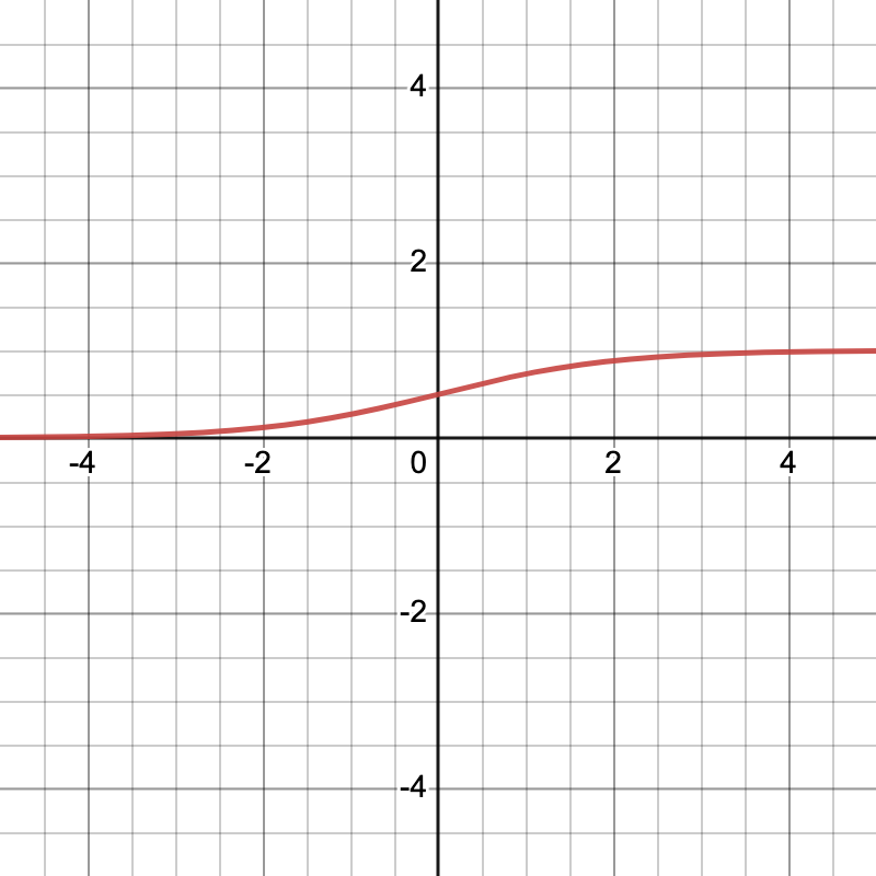
A typical graph of \(P(t) = \dfrac{A}{1 + Me^{-kt}}\) has an S-shape (sigmoidal curve) that rises from near \(0\) as \(t \to -\infty\) to the value \(A\) as \(t \to \infty\text{.}\) The parameter \(A\) sets the upper asymptote. The parameter \(M\) affects the \(y\)-intercept: since \(P(0) = \frac{A}{1+M}\text{,}\) larger \(M\) gives a lower initial value, producing an effect similar to a horizontal shift. The parameter \(k\) controls the steepness of the transition from the lower asymptote to the upper asymptote.
described in detail following the image
graph of \(P(t)\) for some values of the sliders
3.6.3.b
Answer.
The population appears to grow most rapidly at the midpoint of the transition from near \(0\) to the carrying capacity \(A\text{.}\) This occurs when \(P(t) = \dfrac{A}{2}\text{,}\) that is, at half the carrying capacity.
3.6.3.d
Answer.
\(A = 9\text{,}\) \(M = \frac{7}{2} = 3.5\text{,}\) and \(k = \dfrac{1}{2}\ln\!\left(\dfrac{14}{5}\right) \approx 0.516\text{.}\)


Activity 3.6.4.

3.6.4.a
Answer.
\(A = 11.7\text{,}\) \(M \approx 3.776\text{,}\) and \(k = -\frac{1}{3}\ln(0.421) \approx 0.289.\)
3.6.4.b
Answer.
The average rates of change are: \(AV_{[0,2]} \approx 0.650\text{,}\) \(AV_{[2,4]} \approx 0.796\text{,}\) \(AV_{[4,6]} \approx 0.836\text{,}\) \(AV_{[6,8]} \approx 0.747\) thousand animals per year. These represent the average rate at which the population grows on each interval.

4 Trigonometry
4.1 Right triangles
4.1.2 The geometry of triangles


Activity 4.1.2.

4.1.2.a
Answer.
Both triangles share the angle \(\theta\) at vertex \(O\text{,}\) and both have a right angle (\(\angle OPQ\) and \(\angle ONM\)). Since two pairs of angles are equal, the triangles are similar by AA similarity.
4.1.2.b
Answer.
The ratio \(\frac{OP}{OM} = r\text{,}\) so \(\frac{OQ}{ON} = r\) and \(\frac{PQ}{MN} = r\text{.}\)

4.1.3 Ratios of sides in right triangles


Activity 4.1.3.

4.1.3.a
Answer.
With hypotenuse \(7\) and non-right angle \(\theta = \frac{\pi}{7}\text{,}\) the adjacent leg is \(x = 7\cos\left(\frac{\pi}{7}\right) \approx 6.3\text{,}\) the opposite leg is \(y = 7\sin\left(\frac{\pi}{7}\right) \approx 3.0\text{,}\) and the other non-right angle is \(\phi = \frac{\pi}{2} - \frac{\pi}{7} = \frac{5\pi}{14}\text{.}\)
4.1.3.b
Answer.
Without a specific side length, we can only determine that the triangle is similar to a 3-4-5 right triangle: sides are \(3a\text{,}\) \(4a\text{,}\) \(5a\) for some \(a > 0\text{.}\) The angles are \(\alpha = \arcsin\left(\frac{3}{5}\right) \approx 0.6435\) and \(\frac{\pi}{2} - \alpha \approx 0.9273\) radians.
4.1.3.c
Answer.
With angle \(\beta = 1.2\) radians and hypotenuse \(2.7\text{:}\) adjacent leg \(x = 2.7\cos(1.2) \approx 0.98\text{,}\) opposite leg \(y = 2.7\sin(1.2) \approx 2.5\text{,}\) and other angle \(\alpha = \frac{\pi}{2} - 1.2 \approx 0.371\) radians.
4.1.3.d
Answer.
With hypotenuse \(13\) and one leg \(6.5\text{,}\) the other leg is \(\sqrt{13^2 - 6.5^2} = \sqrt{169 - 42.25} \approx 11.26\text{.}\) The angles are \(\arccos\left(\frac{6.5}{13}\right) = \arccos\left(\frac{1}{2}\right) = \frac{\pi}{3} \approx 1.047\) and \(\arcsin\left(\frac{1}{2}\right) = \frac{\pi}{6} \approx 0.524\) radians.
4.1.3.e
Answer.
With legs \(5\) and \(12\text{,}\) the hypotenuse is \(\sqrt{5^2 + 12^2} = \sqrt{169} = 13\text{.}\) The angles are \(\arctan\left(\frac{5}{12}\right) \approx 0.395\) and \(\arctan\left(\frac{12}{5}\right) \approx 1.176\) radians.
4.1.3.f
Answer.
With angle \(\beta = \frac{\pi}{5}\) and opposite leg \(4\text{:}\) \(\sin\left(\frac{\pi}{5}\right) = \frac{4}{h}\) where \(h\) is the hypotenuse, so \(h = \frac{4}{\sin(\pi/5)} \approx 6.805\text{.}\) The adjacent leg is \(\sqrt{h^2 - 16} \approx 5.505\text{.}\) The other angle is \(\frac{\pi}{2} - \frac{\pi}{5} = \frac{3\pi}{10}\text{.}\)

4.1.4 Using a ratio involving sine and cosine


Activity 4.1.4.

Answer.
The river is approximately \(75.256\) meters wide. We could also determine the hypotenuse and the missing non-right angle.

4.2 The Tangent Function
4.2.4 Using the tangent function in right triangles


Activity 4.2.2.

Answer.
The cables have to be about \(418.76\) feet long, anchored about \(353.18\) feet away from the base of the tower.


Activity 4.2.4.

4.2.4.d
Answer.
\(x = \dfrac{1000\tan(19^\circ)}{\tan(25^\circ) - \tan(19^\circ)} \approx 3412.527\)

4.3 Inverses of trigonometric functions
4.3.2 The arccosine function


Activity 4.3.2.

4.3.3 The arcsine function


Activity 4.3.3.

4.3.3.a
Answer.
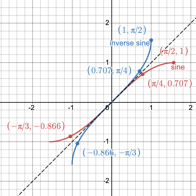
The domain of \(\arcsin\) is \([-1, 1]\) and the range is \(\left[-\frac{\pi}{2}, \frac{\pi}{2}\right]\text{.}\)
4.3.3.b
Answer.
\(\arcsin(-1) = -\frac{\pi}{2}\text{,}\) \(\arcsin\!\left(-\frac{\sqrt{2}}{2}\right) = -\frac{\pi}{4}\text{,}\) \(\arcsin(0) = 0\text{,}\) \(\arcsin\!\left(\frac{1}{2}\right) = \frac{\pi}{6}\text{,}\) and \(\arcsin\!\left(\frac{\sqrt{3}}{2}\right) = \frac{\pi}{3}\text{.}\)
4.3.3.d
Answer.
False. Since \(\sin(5\pi) = 0\) and \(\arcsin(0) = 0\text{,}\) we have \(\arcsin(\sin(5\pi)) = 0 \ne 5\pi\text{.}\)

4.3.4 The arctangent function


Activity 4.3.4.

4.3.4.a
Answer.
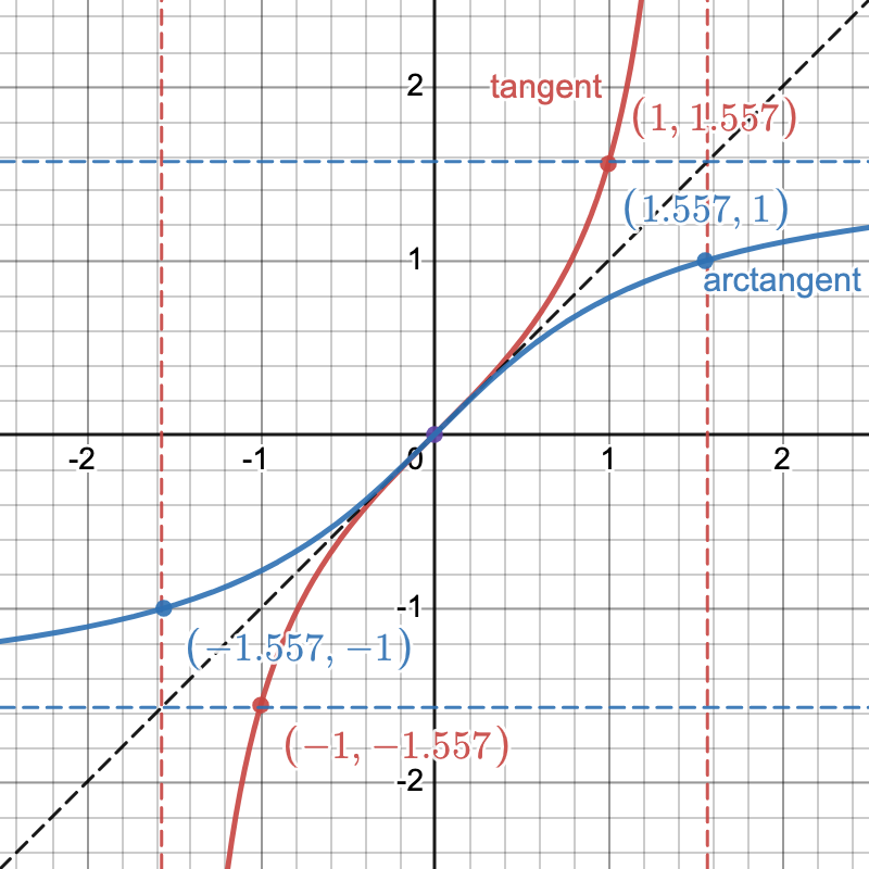
The domain of the arctangent function is all real numbers \((-\infty, \infty)\text{,}\) and the range is the open interval \(\left(-\frac{\pi}{2}, \frac{\pi}{2}\right)\text{.}\)
4.3.4.b
Answer.
\(\arctan(-\sqrt{3}) = -\frac{\pi}{3}\text{,}\) \(\arctan(-1) = -\frac{\pi}{4}\text{,}\) \(\arctan(0) = 0\text{,}\) and \(\arctan\!\left(\frac{1}{\sqrt{3}}\right) = \frac{\pi}{6}\text{.}\)
4.3.4.d
Answer.
As \(t\) increases without bound, \(\arctan(t)\) approaches \(\frac{\pi}{2}\text{.}\)

4.4 Finding Angles
4.4.2 Evaluating inverse trigonometric functions


Activity 4.4.2.

4.4.2.a
Answer.
The hypotenuse has length \(\sqrt{11^2 + 13^2} = \sqrt{290}\text{.}\) The angle \(\alpha\) opposite the leg of length \(11\) satisfies \(\alpha = \arcsin\left(\dfrac{11}{\sqrt{290}}\right) = \arccos\left(\dfrac{13}{\sqrt{290}}\right) \approx 0.702\) radians. The angle \(\beta\) opposite the leg of length \(13\) satisfies \(\beta = \arcsin\left(\dfrac{13}{\sqrt{290}}\right) = \arccos\left(\dfrac{11}{\sqrt{290}}\right) \approx 0.869\) radians.
4.4.2.b
Answer.
\(\alpha = \frac{4\pi}{3}\text{.}\) In addition, \(\sin(\alpha) = -\dfrac{\sqrt{3}}{2}\text{.}\)
4.4.2.c
Answer.
\(\beta = \approx 3.041\) radians. In addition, \(\cos(\beta) \approx -0.9950\text{.}\)

4.4.3 Finding angles in applied contexts


Activity 4.4.3.

Answer.
The angle of the roof with the horizontal is \(\arctan\left(\dfrac{7}{12}\right) \approx 30.26^{\circ}\) (exactly \(\arctan\left(\frac{7}{12}\right)\) radians). Alternatively, this angle equals \(\arcsin\left(\dfrac{7}{\sqrt{193}}\right) = \arccos\left(\dfrac{12}{\sqrt{193}}\right)\text{.}\) The angle at the peak of the roof is formed by the two sloping surfaces; since each makes an angle of \(\arctan\left(\frac{7}{12}\right)\) with the horizontal, the ridge angle is \(180^{\circ} - 2\arctan\left(\frac{7}{12}\right) \approx 119.5^{\circ}\text{.}\)


Activity 4.4.4.

Answer.
Throwing to first base. The angle the throw makes with the first base line is \(\arctan\left(\dfrac{80}{90}\right) \approx 41.6^{\circ}\text{,}\) and with the third base line it is \(\arctan\left(\dfrac{90}{80}\right) \approx 48.4^{\circ}\text{.}\)
Throwing to second base. The angle with the first base line is \(\arctan\left(\dfrac{10}{90}\right) \approx 6.3^{\circ}\text{,}\) and with the third base line it is approximately \(83.7^{\circ}\text{.}\)


Activity 4.4.5.

Answer.
For general height \(h\text{,}\) \(\theta(h) = \arctan\left(\dfrac{h}{4000}\right)\text{.}\)
The average rates of change are: \(AV_{[3000,3500]} \approx \frac{0.075}{500} = 1.5 \times 10^{-4}\) rad/ft; \(AV_{[5000,5500]} \approx \frac{0.046}{500} = 9.2 \times 10^{-5}\) rad/ft; \(AV_{[7000,7500]} \approx \frac{0.030}{500} = 6 \times 10^{-5}\) rad/ft. The camera angle is increasing at a decreasing rate as the rocket climbs higher.

4.5 Other Trigonometric Functions and Identities
4.5.2 Ratios in right triangles


Activity 4.5.2.

Answer.
\(\cos(\beta) = -\frac{1}{2}\text{,}\) \(\sin(\beta) = \frac{\sqrt{3}}{2}\text{,}\) \(\csc(\beta) = \frac{2}{\sqrt{3}}\text{,}\) \(\cot(\beta) = -\frac{\sqrt{3}}{3}\text{,}\) \(\tan(\beta) = -\frac{3}{\sqrt{3}}\text{.}\)

4.5.3 Properties of the secant, cosecant, and cotangent functions


Activity 4.5.3.

4.5.3.a
Answer.
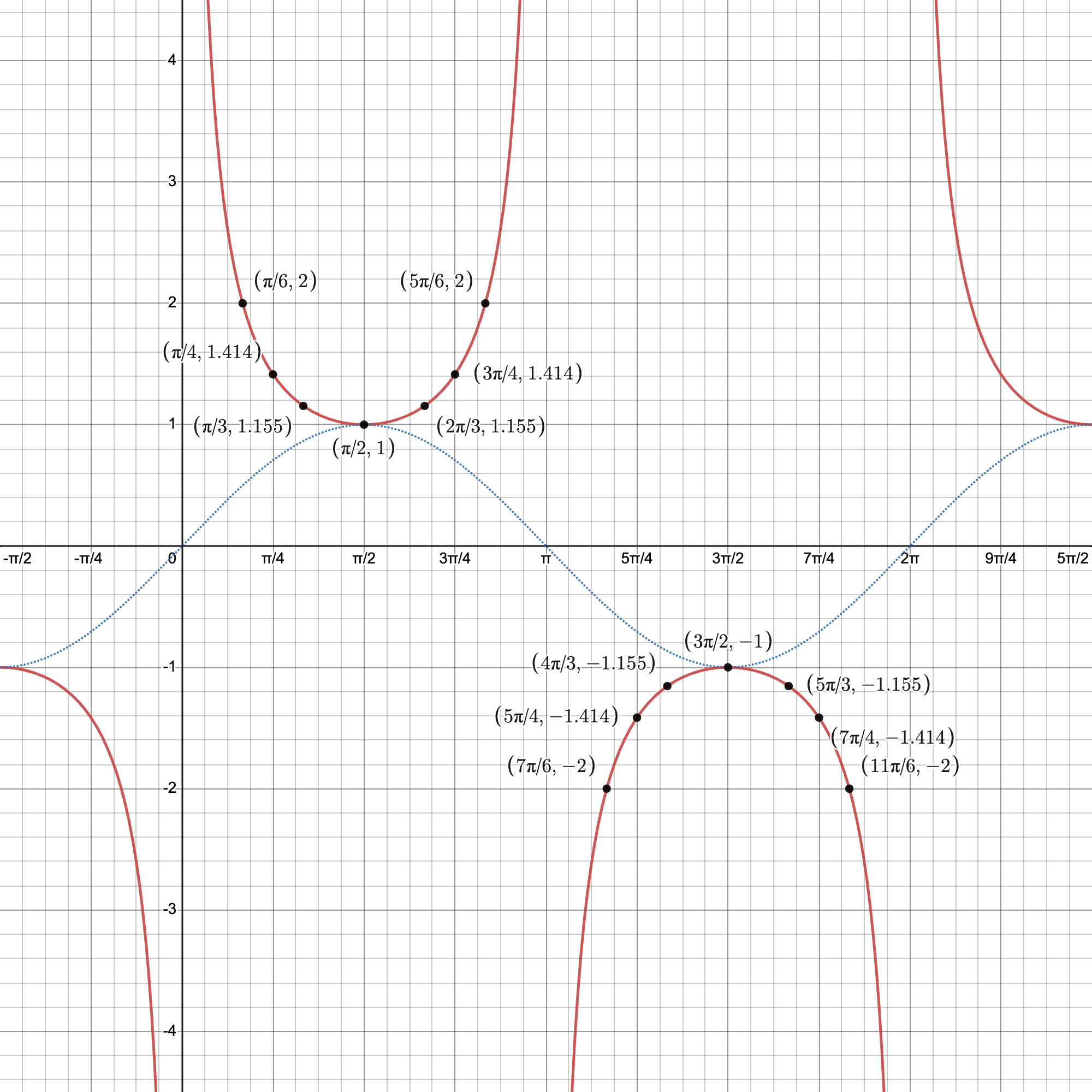
The cosecant values are reciprocals of sine. In Q1 and Q2: \(u, 2, \sqrt{2}, \frac{2\sqrt{3}}{3}, 1, \frac{2\sqrt{3}}{3}, \sqrt{2}, 2, u\text{;}\) In Q3 and Q4: \(-2, -\sqrt{2}, -\frac{2\sqrt{3}}{3}, -1, -\frac{2\sqrt{3}}{3}, -\sqrt{2}, -2, u\text{.}\)
4.5.3.b
Answer.
The cosecant function is positive in quadrants I and II and negative in quadrants III and IV.
4.5.3.d
Answer.
The domain of the cosecant function is all real numbers except integer multiples of \(\pi\text{.}\) The range is \((-\infty, -1] \cup [1, \infty)\text{.}\)


Activity 4.5.4.

4.5.4.a
Answer.
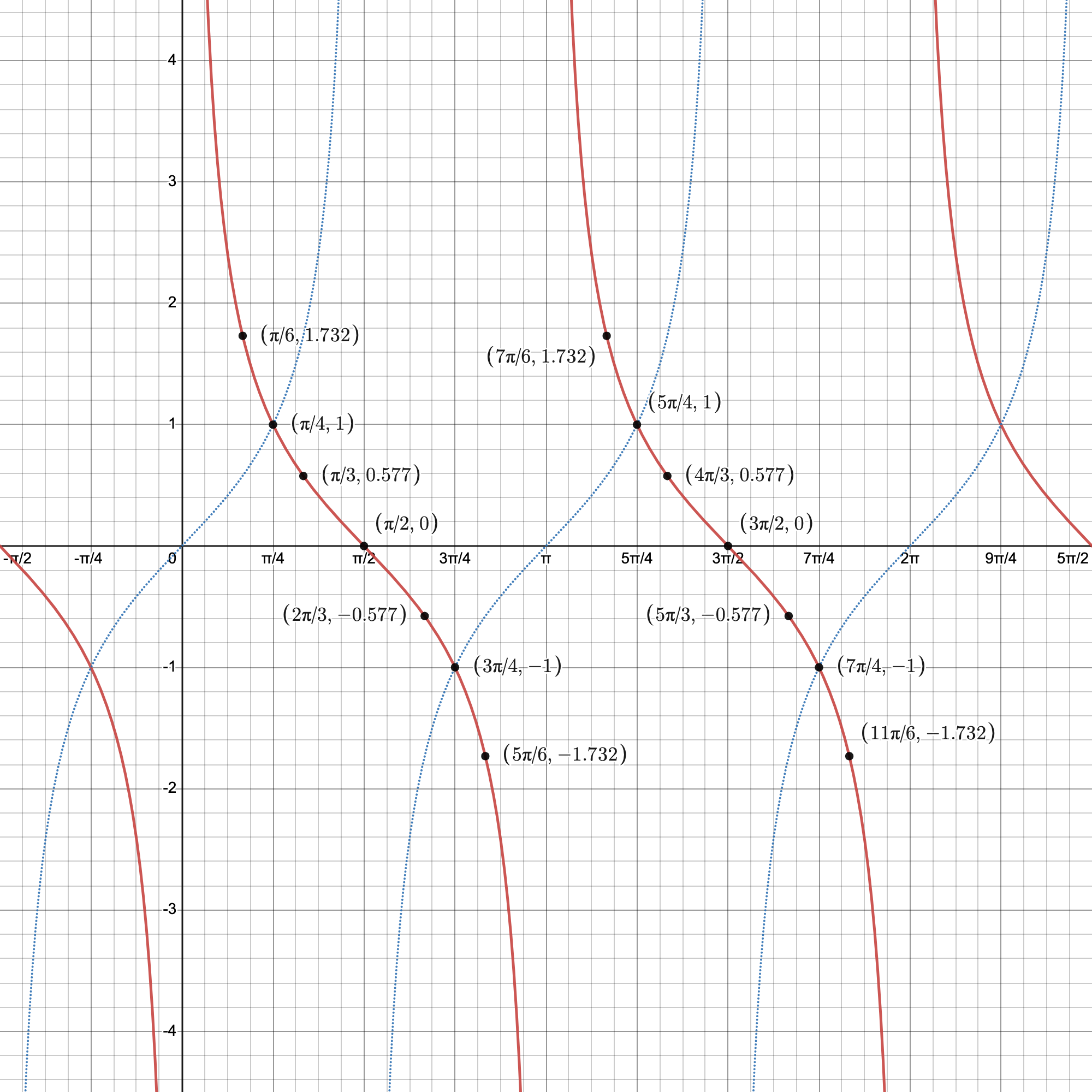
Since \(\cot(t) = \cos(t)/\sin(t)\text{,}\) the cotangent values for Q1 and Q2 are: \(u, \sqrt{3}, 1, \frac{1}{\sqrt{3}}, 0, -\frac{1}{\sqrt{3}}, -1, -\sqrt{3}, u\text{;}\) and for Q3 and Q4: \(\sqrt{3}, 1, \frac{1}{\sqrt{3}}, 0, -\frac{1}{\sqrt{3}}, -1, -\sqrt{3}, u\text{.}\)
4.5.4.b
Answer.
The cotangent function is positive in quadrants I and III and negative in quadrants II and IV.
4.5.4.d
Answer.
The domain of the cotangent function is all real numbers except integer multiples of \(\pi\text{.}\) The range is all real numbers \((-\infty, \infty)\text{.}\)
4.5.4.f
Answer.
The cotangent function is always decreasing on every interval where it is defined.
4.5.4.h
Answer.
The graph of \(r(t) = \cot(t)\) can be obtained from the graph of \(\tan(t)\) by reflecting over the \(y\)-axis and then shifting \(\frac{\pi}{2}\) to the right.

4.5.4 A few important identities


Activity 4.5.5.

4.5.5.c
Answer.
\begin{align*} AV_{[a,a+h]} &= \frac{\sin(a)\cos(h) + \cos(a)\sin(h) - \sin(a)}{h}\\ &= \frac{\sin(a)(\cos(h)-1) + \cos(a)\sin(h)}{h}\\ &= \sin(a) \cdot \frac{\cos(h)-1}{h} + \cos(a) \cdot \frac{\sin(h)}{h} \end{align*}
4.5.5.d
Answer.
As \(h\) approaches 0, the expression \(\dfrac{\cos(h)-1}{h}\) approaches \(0\text{,}\) and \(\dfrac{\sin(h)}{h}\) approaches \(1\text{.}\) Therefore \(AV_{[a,a+h]}\) approaches \(\sin(a) \cdot 0 + \cos(a) \cdot 1 = \cos(a)\text{.}\) This tells us that the instantaneous rate of change of the sine function at \(a\) is \(\cos(a)\text{.}\)

5 Polynomial and Rational Functions
5.1 Infinity, limits, and power functions
5.1.2 Limit notation


Activity 5.1.2.

Answer.
\(f(x)\) \(\lim_{x \to \infty} f(x)\) \(\lim_{x \to -\infty} f(x)\)
\(e^x\) \(\infty\) \(0\)
\(e^{-x}\) \(0\) \(\infty\)
\(\ln(x)\) \(\infty\) not defined
\(x\) \(\infty\) \(-\infty\)
\(x^2\) \(\infty\) \(\infty\)
\(x^3\) \(\infty\) \(-\infty\)
\(x^4\) \(\infty\) \(\infty\)
\(\frac{1}{x}\) \(0\) \(0\)
\(\frac{1}{x^2}\) \(0\) \(0\)
\(\sin(x)\) no limit no limit

5.1.3 Power functions


Activity 5.1.3.

5.1.3.a
Answer.
Two trends to observe: (1) As \(n\) increases, the graph becomes flatter and wider near \(x = 0\) before rising steeply. (2) When \(n\) is even, both ends of the graph go to \(+\infty\) (symmetric about the \(y\)-axis); when \(n\) is odd, the left end goes to \(-\infty\) and the right end goes to \(+\infty\text{.}\)
5.1.3.b
Answer.
On \(0 \lt x \lt 1\text{,}\) the graph of \(x^b\) stays closer to \(0\) than \(x^a\) when \(b \gt a\text{.}\) That is, \(x^a \gt x^b\) on \((0,1)\) when \(a \lt b\text{.}\)
5.1.3.c
Answer.
Two trends to observe: (1) The graphs with even \(n\) are symmetric about the \(y\)-axis, while odd-\(n\) graphs pass through the origin from lower-left to upper-right. (2) For larger \(n\text{,}\) the function stays very close to \(0\) on \((-1,1)\) and then rises very steeply outside that interval.
5.1.3.d
Answer.
On \(x \gt 1\text{,}\) the graph of \(x^b\) lies above the graph of \(x^a\) when \(b \gt a\text{:}\) larger exponents produce faster growth for \(x \gt 1\text{.}\)


Activity 5.1.4.

5.1.4.a
Answer.
Two trends: (1) For even-\(n\) exponents (like \(x^{-2}, x^{-4}, \ldots\)), the graph is symmetric about the \(y\)-axis and stays positive; for odd exponents (like \(x^{-1}, x^{-3}, \ldots\)), the graph is negative for \(x \lt 0\) and positive for \(x \gt 0\text{.}\) (2) As the exponent becomes more negative, the graph becomes more sharply β€œL-shaped” near \(x = 0\text{.}\)
5.1.4.b
Answer.
On \(x \gt 1\text{,}\) \(x^a \lt x^b\) when \(a \lt b\) (with both negative). For example, \(x^{-3} \lt x^{-2}\) for \(x \gt 1\text{,}\) since dividing by a higher power gives a smaller result.
5.1.4.c
Answer.
On \(0 \lt x \lt 1\text{,}\) the situation reverses: \(x^a \gt x^b\) when \(a \lt b\) (i.e., more negative exponents give larger values on \((0,1)\) since dividing by a small number raised to a high power gives a large result).
5.1.4.d
Answer.
Two trends with the wider window: (1) The graphs with even exponents are symmetric about the \(y\)-axis; odd-exponent graphs are antisymmetric. (2) As the exponent becomes more negative, the function rises more steeply near \(x = 0\) (steeper asymptotic behavior).
5.1.4.e
Answer.
As \(x \to \infty\text{,}\) \(x^n \to \infty\) for any positive integer \(n\text{,}\) so \(\frac{1}{x^n} = x^{-n} \to 0\text{.}\) Dividing \(1\) by an ever-larger number drives the result to \(0\text{.}\)

5.2 Polynomials
5.2.2 Key results about polynomial functions


5.2.3 Using zeros and signs to understand polynomial behavior


Activity 5.2.3.

5.2.3.c
Answer.
The real zeros are \(x = -1520\text{,}\) \(x = 3471\text{,}\) and \(x = 9738\text{.}\)
5.2.3.e
Answer.
The graph is positive (above the \(x\)-axis) for \(x \lt -1520\text{,}\) crosses zero at \(x=-1520\) (passes through), touches zero at \(x=3471\) (bounce, even multiplicity), remains negative until \(x=9738\text{,}\) then crosses zero and becomes positive. The leading term \(4692 x^6\) means both ends go to \(+\infty\text{.}\)
5.2.3.f
Answer.
Using a graphing utility, the zeros at \(x=-1520\text{,}\) \(3471\text{,}\) and \(9738\) are spread over a large \(x\)-range, making it challenging to see all features at once. It is difficult to tell from the graph that \(x=3471\) is a bounce point (touching zero without crossing) unless the scale is set appropriately.

5.2.4 Multiplicity of polynomial zeros


Activity 5.2.4.

5.2.4.a
Answer.
One formula: \(f(x) = -21\left(\dfrac{x+12}{12}\right)^3\left(\dfrac{x+9}{9}\right)^2\left(\dfrac{x-4}{4}\right)^4\left(\dfrac{x-10}{10}\right)\)
5.2.4.b
Answer.
One example is: \(p(x) = -2\left(\dfrac{x+8}{8}\right)^2\left(\dfrac{x+4}{4}\right)^3(x-1)\left(\dfrac{x-5}{5}\right)^2\left(\dfrac{x-7.5}{7.5}\right)\)
5.2.4.c
Answer.
One example: \(q(x) = -10\left(\dfrac{x+2}{2}\right)^4\left(\dfrac{x-3}{3}\right)\left(\dfrac{x-9}{9}\right)^3\)

5.3 Modeling with polynomial functions
5.3.2 Volume, surface area, and constraints


5.3.3 Other applications of polynomial functions


Activity 5.3.4.

5.3.4.d
Answer.
Each additional term in the polynomial extends the range of \(x\)-values over which the approximation is accurate. \(T_{19}(x)\) provides an excellent approximation to \(\sin(x)\) over a very large interval, essentially indistinguishable from \(\sin(x)\) on most standard viewing windows.
5.3.4.e
Answer.
Following the pattern of alternating signs and even powers, the next polynomials are
\begin{align*} P_6(x) &= 1 - \frac{x^2}{2!} + \frac{x^4}{4!} - \frac{x^6}{6!},\\ P_8(x) &= 1 - \frac{x^2}{2!} + \frac{x^4}{4!} - \frac{x^6}{6!} + \frac{x^8}{8!},\\ P_{18}(x) &= \sum_{j=0}^{9} \frac{(-1)^j x^{2j}}{(2j)!}. \end{align*}
Polynomial approximations can approximate \(y = \cos(x)\) just as well as \(y = \sin(x)\text{;}\) each added term extends the range of accuracy.

5.4 Rational Functions
5.4.2 Long-range behavior of rational functions


Activity 5.4.2.

5.4.2.a
Answer.
\(r(x)=\frac{3 - \frac{5}{x} + \frac{1}{x^2}}{7 + \frac{2}{x} - \frac{11}{x^2}}\)
5.4.2.d
Answer.
The graph of \(r\) approaches the horizontal line \(y = \dfrac{3}{7}\) as \(x \to \pm\infty\text{.}\) This line is called a horizontal asymptote of \(r\text{.}\) The limits found in (b) and (c) say that far to the left and far to the right of the origin, \(r(x)\) gets arbitrarily close to \(\dfrac{3}{7}\text{.}\)


Activity 5.4.3.

5.4.3.a
Answer.
As \(x \to \infty\text{,}\) the numerator \(\to 0\) and the denominator \(\to 7\text{,}\) so \(\displaystyle\lim_{x \to \infty} s(x) = 0\text{.}\)
5.4.3.b
Answer.
The graph of \(y = s(x)\) has a horizontal asymptote at \(y = 0\text{.}\) Far to the left and right, \(s(x)\) approaches the \(x\)-axis. This occurs because the denominator grows much faster than the numerator (degree 2 vs. degree 1).
5.4.3.c
Answer.
As \(x \to \infty\text{,}\) the numerator \(\to 3\) and the denominator \(\to 0^+\text{,}\) so \(\displaystyle\lim_{x \to \infty} u(x) = +\infty\text{.}\)
5.4.3.d
Answer.
The graph of \(y = u(x)\) increases without bound as \(x \to \infty\text{;}\) \(u\) has no horizontal asymptote.

5.4.3 The domain of a rational function


Activity 5.4.4.

5.4.4.c
Answer.
The domain of \(h\) is all real numbers except \(x = 0\text{,}\) \(x = 1\text{,}\) and \(x = 2\text{.}\)
5.4.4.d
Answer.
The domain of \(j\) is all real numbers except \(x = -1\text{,}\) \(x = -3\text{,}\) and \(x = 5\text{.}\)
5.4.4.e
Answer.
The domain of \(k\) is all real numbers except \(x = -2\text{,}\) \(x = 0\text{,}\) and \(x = 2\text{.}\)
5.4.4.f
Answer.
The domain of \(m\) is all real numbers except \(x = -1\text{,}\) \(x = 2\text{,}\) and \(x = 3\text{.}\)

5.4.4 Applications of rational functions


Activity 5.4.5.

5.4.5.a
Answer.
The box has a shorter base side of length \(x\text{,}\) a longer base side of length \(2x\text{,}\) and height \(h\text{.}\)
5.4.5.b
Answer.
The volume is \(V = 2x^2 h\text{.}\) Setting \(V = 15\) gives \(h = \dfrac{15}{2x^2}\text{.}\)
5.4.5.f
Answer.
From a graph of \(S(x) = 2x^2 + \dfrac{45}{x}\) on \((0, \infty)\text{,}\) the minimum value of \(S\) occurs at approximately \(x \approx 2.24\) feet, giving a minimum surface area of approximately \(S \approx 30.0\) square feet.

5.5 Key features of rational functions
5.5.2 When a rational function has a β€œhole”


Activity 5.5.2.

5.5.3 Sign charts and finding formulas for rational functions


Activity 5.5.3.

5.5.3.c
Answer.
One formula consistent with these features is \(w(x) = \frac{9(x+4)(x-5)^2}{50(x+1)^2(x-3)}.\)