We start with an easy problem. An object travels in a straight line at a constant velocity of 5 ft⁄s for 10 seconds. How far away from its starting point is the object?
We approach this problem with the familiar “\(\text{Distance } = \text{ Rate } \times \text{ Time}\)” equation. In this case, the distance traveled is 5 ft⁄s×10 s\(= 50\) feet.
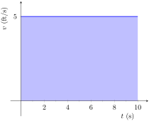
It is interesting to note that this solution of 50 feet can be represented graphically. Consider Figure 5.2.2, where the constant velocity of 5 ft⁄s is graphed on the axes. Shading the area under the line from \(t=0\) to \(t=10\) gives a rectangle with an area of 50 square units; when one considers the units of the axes, we can say this area represents 50 ft.
The \(y\) axis is drawn from \(0\) to \(5\) represents velocity in feets per second and the \(x\) axis is drawn from \(0\) to \(10\) represents time in second. The function \(y=5\) for all values of \(x\) until \(10\text{,}\) the function is a straight line parallel to the \(x\) axis. The area under the line to the \(x\) axis is shaded, and is drawn between \(x=0\) and \(x=10\text{.}\)
Now consider a slightly harder situation (and not particularly realistic): an object travels in a straight line with a constant velocity of 5 ft⁄s for 10 seconds, then instantly reverses course at a rate of 2 ft⁄s for 4 seconds. (Since the object is traveling in the opposite direction when reversing course, we say the velocity is a constant -2 ft⁄s.) How far away from the starting point is the object — what is its displacement?
Two instruments that can be found in any car are the odometer, which displays distance traveled, and the speedometer, which displays the speed at which you are traveling.
Imagine you are driving a car in which the odometer is broken, but you have a passenger who is willing to record your speed at regular intervals of time.
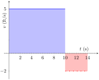
We can again depict this situation graphically. In Figure 5.2.5 we have the velocities graphed as straight lines on \([0,10]\) and \([10,14]\text{,}\) respectively. The displacement of the object is
The \(y\) axis is drawn from \(0\) to \(5\) represents velocity in feets per second and the \(x\) axis is drawn from \(0\) to \(14\) represents time in seconds. There are two areas in the graph both rectangular in shape, the bigger one lies in the first quadrant and the smaller one lies in the fourth quadrant. The function \(y=5\) is a straight line parallel to the \(x\) axis and creates the bigger area under graph, and is drawn between \(x=0\) and \(x=10\text{.}\) The function \(y=-2\text{,}\) is a straight line parallel to the \(x\) axis and creates the smaller area, and is drawn between \(x=10\) and \(x = 14\text{.}\)
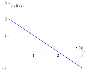
The velocity of an object moving straight up/down under the acceleration of gravity is given as \(v(t) = -32t+48\text{,}\) where time \(t\) is given in seconds and velocity is in ft⁄s. When \(t=0\text{,}\) the object had a height of 0 ft.
To answer questions about the height of the object, we need to find the object’s position function \(s(t)\text{.}\) This is an initial value problem, which we studied in the previous section. We are told the initial height is \(0\text{,}\) i.e., \(s(0) = 0\text{.}\) We know \(s'(t) = v(t) = -32t+48\text{.}\) To find \(s\text{,}\) we find the indefinite integral of \(v(t)\text{:}\)
To find the maximum height of the object, we need to find the maximum of \(s\text{.}\) Recalling our work finding extreme values, we find the critical points of \(s\) by setting its derivative (the velocity function) equal to \(0\) and solving for \(t\text{:}\)
\begin{align*}
0 \amp = -32t+48\\
t \amp =48/32\\
\amp = 1.5\text{ s }\text{.}
\end{align*}
(Notice how we ended up just finding when the velocity was 0ft/s!) The first derivative test shows this is a maximum, so the maximum height of the object is found at
\begin{equation*}
s(1.5) = -16(1.5)^2+48(1.5)=36\text{ ft }\text{.}
\end{equation*}
While we have answered all three questions (using derivatives and antiderivatives), let’s look at them again graphically, using the concepts of area that we explored earlier.
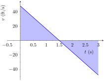
Figure 5.2.7 shows a graph of \(v(t)\) on axes from \(t=0\) to \(t=3\text{.}\) It is again straightforward to find \(v(0)\text{.}\) How can we use the graph to find the maximum height of the object?
The \(y\) axis is drawn from \(-40\) to \(40\) and the \(x\) axis is drawn from \(0\) to \(3\text{.}\) The line starts from point \((0, 48)\) and crosses the \(x\) axis at \(x=1.5\text{,}\) the area under the curve forms a right angled triangle in the first quadrant with the positive \(x\) and \(y\) axes. After crossing the \(x\) axis at \(x=1.5\) the line goes down to point \((3,-48)\text{.}\) Another right angle is formed on the \(x\) axis but in the fourth quadrant with the \(x\) axis and line \(x=3\text{.}\)
Recall how in our previous work that the displacement of the object (in this case, its height) was found as the area under the velocity curve, as shaded in the figure. Moreover, the area between the curve and the \(t\)-axis that is below the \(t\)-axis counted as “negative” area. That is, it represents the object coming back toward its starting position. So to find the maximum distance from the starting point — the maximum height — we find the area under the velocity line that is above the \(t\)-axis, i.e., from \(t=0\) to \(t=1.5\text{.}\) This region is a triangle; its area is
\begin{align*}
\text{ Area } \amp = \frac12\text{ Base } \times \text{ Height }\\
\amp =\frac12\times 1.5\text{ s } \times 48\text{ ft/s }\\
\amp = 36\text{ ft }
\end{align*}
which matches our previous calculation of the maximum height.
Finally, to find the height of the object at time \(t=2\) we calculate the total “signed area” (where some area is negative) under the velocity function from \(t=0\) to \(t=2\text{.}\) This signed area is equal to \(s(2)\text{,}\) the displacement (i.e., signed distance) from the starting position at \(t=0\) to the position at time \(t=2\text{.}\) That is,
Notice how we answered each question in this example in two ways. Our first method was to manipulate equations using our understanding of antiderivatives and derivatives. Our second method was geometric: we answered questions looking at a graph and finding the areas of certain regions of this graph.
The above example does not prove a relationship between area under a velocity function and displacement, but it does imply a relationship exists. Section 5.4 will fully establish fact that the area under a velocity function is displacement.
Given a graph of a function \(y=f(x)\text{,}\) we will find that there is great use in computing the area between the curve \(y=f(x)\) and the \(x\)-axis. Because of this, we need to define some terms.
By our definition, the definite integral gives the “signed area under \(f\text{.}\)” We usually drop the word “signed” when talking about the definite integral, and simply say the definite integral gives “the area under \(f\)” or, more commonly, “the area under the curve.”
The previous section introduced the indefinite integral, which related to antiderivatives. We have now defined the definite integral, which relates to areas under a function. The two are very much related, as we’ll see when we learn the Fundamental Theorem of Calculus in Section 5.4. Recall that earlier we said that the “\(\int\)” symbol was an “elongated S” that represented finding a “sum.” In the context of the definite integral, this notation makes a bit more sense, as we are adding up areas under the function \(f\text{.}\)
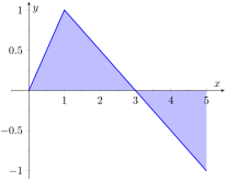
The \(y\) axis is drawn between \(-1\) to \(1\) and the \(x\) axis is drawn between \(0\) to \(5\text{.}\) There is a triangle in the first quadrant drawn on the \(x\) axis with its base from \(x=0\) to \(x=3\) the peak of the triangle is at point \((1,1)\text{.}\) The area in the first quadrant is the shaded portion inside the triangle.
The second area is a right angle triangle and is drawn on the \(x\) axis between \(x=3\) and \(x=5\text{.}\) The triangle lies in the fourth quadrant with its peak at point \((5,-1)\) and the function forming the hypotenuse.
\(\int_0^3 f(x)\, dx\) is the area under \(f\) on the interval \([0,3]\text{.}\) This region is a triangle, so the area is \(\int_0^3 f(x)\, dx=\frac12(3)(1) = 1.5\text{.}\)
\(\int_3^5 f(x)\, dx\) represents the area of the triangle found under the \(x\)-axis on \([3,5]\text{.}\) The area is \(\frac12(2)(1) = 1\text{;}\) since it is found under the \(x\)-axis, this is “negative area.” Therefore \(\int_3^5 f(x)\, dx = -1\text{.}\)
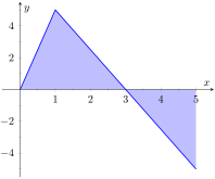
\(\int_0^35f(x)\, dx\) is the area under \(5f\) on \([0,3]\text{.}\) This is sketched in Figure 5.2.12. Again, the region is a triangle, with height 5 times that of the height of the original triangle. Thus the area is \(\int_0^35f(x)\, dx = \frac12(15)(1) = 7.5\text{.}\)
\(\int_1^1f(x)\, dx\) is the area under \(f\) on the “interval” \([1,1]\text{.}\) This describes a line segment, not a region; it has no width. Therefore the area is 0.
The \(y\) axis is drawn between \(-5\) to \(5\) and the \(x\) axis is drawn between \(0\) to \(5\text{.}\) There is a triangle in the first quadrant drawn on the \(x\) axis with its base from \(x=0\) to \(x=3\) the peak of the triangle is at point \((1,5)\text{.}\) The area in the first quadrant is the shaded portion inside the triangle.
Let \(f\) and \(g\) be defined on a closed interval \(I\) that contains the values \(a\text{,}\)\(b\) and \(c\text{,}\) and let \(k\) be a constant. The following hold:
The graph in Figure 5.2.5 shows the signed area under the graph of a piecewise-defined function with a jump discontinuity. Which of the properties in Theorem 5.2.13 best enables us to evaluate the integral of this function?
This states that total area is the sum of the areas of subregions. It is easily considered when we let \(a\lt b\lt c\text{.}\) We can break the interval \([a,c]\) into two subintervals, \([a,b]\) and \([b,c]\text{.}\) The total area over \([a,c]\) is the area over \([a,b]\) plus the area over \([b,c]\text{.}\) It is important to note that this still holds true even if \(a\lt b\lt c\) is not true. We discuss this in the next point.
This property can be viewed a merely a convention to make other properties work well. (Later we will see how this property has a justification all its own, not necessarily in support of other properties.) Suppose \(b\lt a\lt c\text{.}\) The discussion from the previous point clearly justifies
Property \((3)\) justifies changing the sign and switching the bounds of integration on the \(\ds -\int_b^a f(x)\, dx\) term; when this is done, Equations (5.2.1) and (5.2.2) are equivalent. The conclusion is this: by adopting the convention of Property (3), Property (2) holds no matter the order of \(a\text{,}\)\(b\) and \(c\text{.}\) Again, in the next section we will see another justification for this property.
Each of these may be non-intuitive. Property (5) states that when one scales a function by, for instance, 7, the area of the enclosed region also is scaled by a factor of 7. Both Properties (4) and (5) can be proved using geometry. The details are not complicated but are not discussed here.
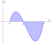
The \(x\) and the \(y\) axes are uncalibrated, there are three positions \(a\text{,}\)\(b\) and \(c\) in order on the \(x\) axis where the inflection changes. The curve in the first quadrant is smaller, the area under the curve forms a bell jar shape it extends from \(x=a\) to \(x=b\text{.}\) The other curve is twice in height as the first and lies in the fourth quadrant. It is also bell jar shaped, but is inverted on the positive \(x\) axis and extends between \(x=b\) to \(x=c\text{.}\)
\(\int_a^b f(x)\, dx\) has a positive value (since the area is above the \(x\)-axis) whereas \(\int_b^c f(x)\, dx\) has a negative value. Hence \(\int_a^b f(x)\, dx\) is bigger.
\(\int_a^c f(x)\, dx\) is the total signed area under \(f\) between \(x=a\) and \(x=c\text{.}\) Since the region below the \(x\)-axis looks to be larger than the region above, we conclude that the definite integral has a value less than 0.
Note how the second integral has the bounds “reversed.” Therefore \(\int_c^b f(x)\, dx=-\int_b^c f(x)\, dx\) represents a positive number, greater than the area described by the first definite integral. Hence \(\int_c^b f(x)\, dx\) is greater.
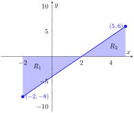
It is useful to sketch the function in the integrand, as shown in Figure 5.2.19. We see we need to compute the areas of two regions, which we have labeled \(R_1\) and \(R_2\text{.}\) Both are triangles, so the area computation is straightforward:
The \(y\) axis is drawn from \(-10\) to \(10\) and the \(x\) axis is drawn from \(-3\) to \(5\text{.}\) The function is a straight line that starts from point \((-2,-8)\) and ends at point \((5,6)\text{.}\) The function intersects the \(x\) axis at \(x=2\text{.}\)
The function, below the \(x\) axis creates a right angled triangle with the \(x\) axis and line \(x=-2\) from \(y=0\) to \(y=-8\text{,}\) with its base from \(x=-2\) to \(x=2\text{.}\) This area is named R1.
The function above the \(x\) axis forms a right angled triangle with the \(x\) axis and line \(x=5\) from \(y=0\) to \(y=6\text{,}\) with its base from \(x=2\) and \(x=5\text{.}\) This area is named R2.
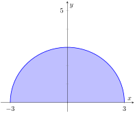
The graph shows the area under the curve that is a semicircle with radius \(3\) on the \(x\) axis with centre at origin. It lies on the first and the second quadrant.
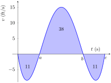
Consider the graph of a velocity function of an object moving in a straight line, given in Figure 5.2.22, where the numbers in the given regions gives the area of that region. Assume that the definite integral of a velocity function gives displacement. Find the maximum speed of the object and its maximum displacement from its starting position.
The \(y\) axis is drawn from \(-10\) to \(15\) and it represents velocity in feets per second, the \(x\) axis is uncalibrated and represents time in seconds. There are three points on the \(x\) axis marked \(a\text{,}\)\(b\) and \(c\) in that order.
In the fourth quadrant, on the \(x\) axis from \(0\) to \(a\text{,}\) a parabola is drawn with its peak at \(y=-10\text{.}\) The number \(11\) is written inside the shaded portion.
From \(b\) to \(c\) the third parabola is located in the fourth quadrant with its peak at \(x=-10\text{,}\) the number \(11\) is written inside it, indicating same size as the first parabola.
At time \(t=0\text{,}\) the displacement is 0; the object is at its starting position. At time \(t=a\text{,}\) the object has moved backward 11 feet. Between times \(t=a\) and \(t=b\text{,}\) the object moves forward 38 feet, bringing it into a position 27 feet forward of its starting position. From \(t=b\) to \(t=c\) the object is moving backwards again, hence its maximum displacement is 27 feet from its starting position.
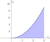
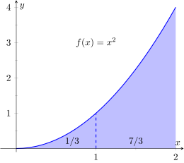
In our examples, we have either found the areas of regions that have nice geometric shapes (such as rectangles, triangles and circles) or the areas were given to us. Consider Figure 5.2.23, where a region below \(y=x^2\) is shaded. What is its area? The function \(y=x^2\) is relatively simple, yet the shape it defines has an area that is not simple to find geometrically.
The \(y\) axis is drawn from \(0\) to \(10\) and the \(x\) axis is drawn from \(0\) to \(3\text{.}\) The curve is drawn in the first quadrant, it starts at the origin and increases gently until \(x=1\) and steeply from \(x=1\) to \(x=3\) and ends at point \((3,9)\text{.}\)
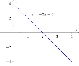
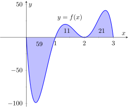
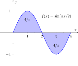
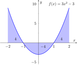
A graph of a function \(f(x)\) is given; the numbers inside the shaded regions give the area of that region. Evaluate the definite integrals using this area information.