
3.2. Optimization Using Solver
A lot of data science and machine learning concerns itself with optimization. In the business world, people are often trying to maximize profit and/or minimize costs. In the manufacturing world, people are often trying to figure out how to make the best product while using the least amount of resources. Machine learning algorithms are trying to figure out how to make the best predictions while minimizing the error in those predictions. At the same time, all of these problems come with a set of constraints. You don’t have unlimited money or inventory or time to do all of the things you want to do. These problems are hard to solve in your head, as there are too many things to think about at once, and when you change one thing, that very often impacts another thing.
Some key terminology to understand:
Objective function: This is the thing you want to minimize or maximize. For example, you might want to maximize the total profit. Or, you might want to minimize the total cost.
Constraints: You can think of constraints as the rules you must follow. You can’t sell more things than you have. You can’t spend more money than you have in the bank. You can only make so many pizzas every hour.
Google Sheets has an excellent plugin that allows you to solve these kinds of optimization problems. Let’s look at an example problem to get an idea of what Solver can do for us.
Suppose you run a lemonade stand on the corner of your street. In addition to lemonade, you also sell the items in the table below. This is a pretty advanced lemonade stand! But, of course, you are a college student, not a six year old.
Item |
Cost |
Sale Price |
Inventory |
lemonade |
0.25 |
1.25 |
500 |
candy bar |
0.5 |
1.25 |
50 |
popcorn |
0.1 |
1.5 |
300 |
licorice |
0.35 |
0.75 |
50 |
pizza slice |
0.825 |
2 |
80 |
burger |
1 |
4.5 |
80 |
cheese curds |
0.75 |
3 |
50 |
chips |
0.25 |
0.8 |
100 |
Being a student of data science, you want to figure out how to maximize your profits from the lemonade stand. You have the following inventory on hand, but because of your busy schedule, you know that you can only sell 500 items before you close up shop for the day. You are a good salesperson, and can usually get your customers to buy whatever you suggest. So, the question is how to you steer those customers to make the maximum amount of money.
Start by entering the data from the table above into a Google Sheets document. Now, add a column called “profit” and figure out the profit margin for each item. It looks like cheese curds and burgers are your most profitable items. You must be in Wisconsin! But you only have 50 cheese curds and 80 burgers. So you have lots more to sell. Let’s set this up as an optimization problem, and use the Solver tool to find the best answer for us.
Add another column called “numsold” to keep track of how many items you have sold, and another column called “total profit” that multiplies the number sold by the profit for that item. The sum of that column will be your total profit. It is the grand total that we want to maximize. That sum is our objective function.
The next question is: What are our constraints?
You can’t sell more than 500 items total.
You can’t sell more items than you have in your inventory.
Given those constraints, we will use Solver to come up with the following solution.
Item |
Cost |
Price |
Inventory |
Profit |
Numsold |
Total Profit |
lemonade |
0.25 |
1.25 |
500 |
1 |
0 |
0 |
candy bar |
0.5 |
1.25 |
50 |
0.75 |
0 |
0 |
popcorn |
0.1 |
1.5 |
300 |
1.4 |
300 |
420 |
licorice |
0.35 |
0.75 |
50 |
0.4 |
0 |
0 |
pizza slice |
0.825 |
2 |
80 |
1.175 |
70 |
82.25 |
burger |
1 |
4.5 |
80 |
3.5 |
80 |
280 |
cheese curds |
0.75 |
3 |
50 |
2.25 |
50 |
112.5 |
chips |
0.25 |
0.8 |
100 |
0.55 |
0 |
0 |
Grand Total |
500 |
894.75 |
||||
max items |
500 |
The interesting part is that we are going to let Solver fill in the values for us in the numsold column. You should start out by trying out some values for yourself, so you can see the recalculation happening. Now, let’s set up Solver to find the best values for that column.
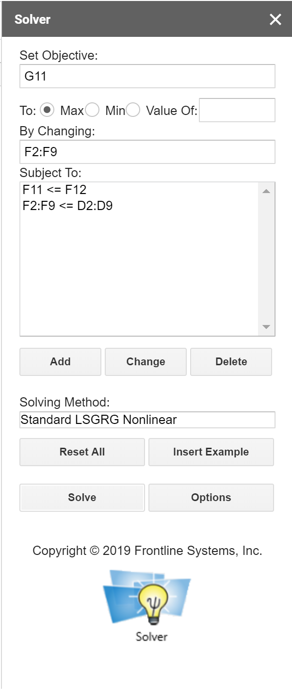
We said that our objective function was to maximize profit. That value is the total that shows up as 894.75 and is in cell G11 in the spreadsheet. So, in our Solver tab in the Set Objective input box, we will set G11 as our objective cell. You can see that at the right. You can also see that we have checked the box to maximize that objective. You can think of Set Objective as the dependent variable.
Next, you can see the By Changing input box. This is where we tell Solver the values it can change. We are allowing Solver to decide how much of each item we should sell. Those are in cells F2:F9. It doesn’t matter if you have already entered a few values into those cells, as Solver will override them. You can think of By Changing as the independent variable.
Finally, we have the Subject To entry area. Recall that our two constraints were that we could not sell more than 500 total items. That means that in our spreadsheet, F11 must be less than or equal to the value in F12. Note that makes it easy for us to change our constraint by just changing the value in cell F12 and rerunning Solver.
Also, we said that you could not sell more items than you have in the inventory. So F2:F9 must be less than or equal to D2:D9.
When you have all of the above, click the “solve” button. You should end up with the same values as shown in the table above.
Now, this model is not very realistic. Let’s add in the fact that you have to operate under a budget, and we will interpret the inventory column to mean the maximum number of a particular item you can sell. The new constraint we will add is that since you are a college student, you only have $50 to spend on supplies. So not only do you have a limit on the number of items you can sell during the time your lemonade stand is open, but you also have a limit on how much you can spend on supplies. Modify the spreadsheet so that you have a new constraint that reflects that you can only spend $50 on your supplies. You may not be surprised to see that when you have such a limited budget, you are forced to focus your sales on the lowest priced highest profit items: lemonade and popcorn.