
5.2. Jupyter Notebooks
The files you will be working with are called Jupyter Notebooks. This comes from the idea of a lab notebook, where you combine figures, data that you have gathered, and explanations about how the data fits the theory. In our case, a notebook can be used to write and run programs and to edit accompanying text. This makes it convenient as a way to deliver some of this course content, but you can also use it to create a report that contains coding (and its output including graphs).
5.2.1. Text Cells
In a notebook, each rectangle containing text or code is called a cell.
Text cells (like the one shown in Figure 1) can be edited by double-clicking on them. They’re written in a format called Markdown. You don’t need to learn Markdown, but you might pick up some aspects of the language from looking at the content that we provide.
After you edit a text cell, click the “run cell” button at the top that looks
like ▶ or hold down shift + return to confirm any changes.
Practice editing a text cell by making any part of the text in the cell that you choose bold. Bold is created in Markdown by surrounding the word or phrase you want bolded with double underscores or double asterisks.
You can also double-click on any text cell that is given to you to see how the authors of the notebook created various bits of styling like italics or inline images like this one that explains the various parts of Jupyter.
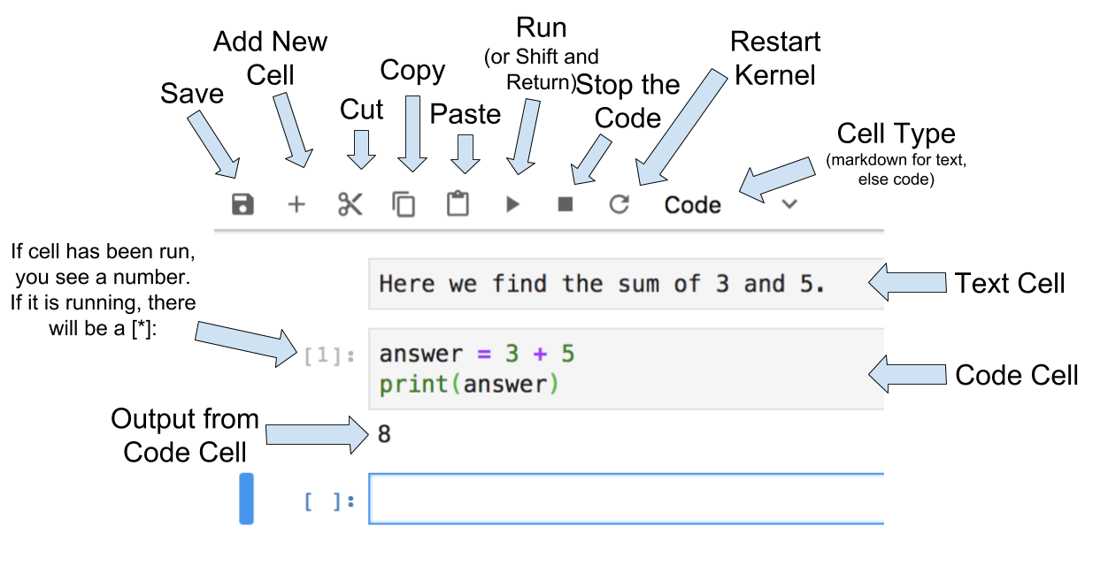
Figure 1: Anatomy of JupyterLab Notebook
5.2.2. Code Cells
Alternatively, cells can contain Python 3 code. Clicking “run cell” for a code cell will execute the content of the cell and print out the output of the code snippet right below the code cell. Try running this cell.
3+5*4%43
23
This doesn’t work just for arithmetic operations but any Python code that you might write.
import math

circle_areas = []

for i in range(1, 5):
    circle_areas.append(math.pi * i**2)

circle_areas
[3.141592653589793, 12.566370614359172, 28.274333882308138, 50.26548245743669]
Notice that if a cell ends with a value by itself on a line, the resulting value gets printed in the output. This doesn’t work if the cell ends with an assignment of a value to a variable.
a = 5
Note that no output is produced when you run the previous cell. However, the
value of a is saved and is available in other cells.
a * a
25
25
This is useful because it means that we can put import statements and the
time-consuming reading of large data sources in one cell (usually) at the start
of the notebook, and experiment with manipulations of that data in later cells
without having the wait to reload the data. The caveat to this is that each cell
is executed when you run it, so you could accidentally or willfully run cells
out of order. Below is an example.
# Run this cell once
my_list = ["red", "green", "blue"]
# Run this cell twice
my_list.append("purple")
# Run this cell once
print(my_list)
['red', 'green', 'blue', 'purple']
Notice that my_list contains “purple” twice even the code above only adds it
once. In general, you should write your code assuming that each cell is run once
from top to bottom. There’s even a menu to help you do that. The “Run” menu has
“Run All Above Selected Cell” and “Run All Cells” functions that allow you to
get your notebook in a predictable state if you ever get confused by having run
cells multiple times or out of order.