7.6. The Shell Sort¶

The shell sort, sometimes called the “diminishing increment sort,” improves on the insertion sort by breaking the original vector into a number of smaller subvectors, each of which is sorted using an insertion sort. The unique way that these subvectors are chosen is the key to the shell sort. Instead of breaking the vector into subvectors of contiguous items, the shell sort uses an increment i, sometimes called the gap, to create a subvector by choosing all items that are i items apart.

This can be seen in Figure 6. This vector has nine items. If we use an increment of three, there are three subvectors, each of which can be sorted by an insertion sort. After completing these sorts, we get the vector shown in Figure 7. Although this vector is not completely sorted, something very interesting has happened. By sorting the subvectors, we have moved the items closer to where they actually belong.

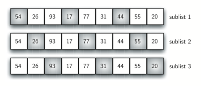
../_images/shellsortA.png — Figure 6: A Shell Sort with Increments of Three¶

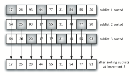
../_images/shellsortB.png — Figure 7: A Shell Sort after Sorting Each subvector¶

Figure 8 shows a final insertion sort using an increment of one; in other words, a standard insertion sort. Note that by performing the earlier subvector sorts, we have now reduced the total number of shifting operations necessary to put the vector in its final order. For this case, we need only four more shifts to complete the process.

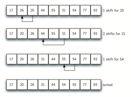
../_images/shellsortC.png — Figure 8: ShellSort: A Final Insertion Sort with Increment of 1¶

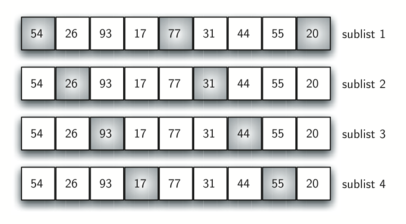
../_images/shellsortD.png — Figure 9: Initial Subvectors for a Shell Sort¶

We said earlier that the way in which the increments are chosen is the unique feature of the shell sort. The function shown in ActiveCode 1 uses a different set of increments. In this case, we begin with \(\frac {n}{2}\) subvectors. On the next pass, \(\frac {n}{4}\) subvectors are sorted. Eventually, a single vector is sorted with the basic insertion sort. Figure 9 shows the first subvectors for our example using this increment.

The following invocation of the shellSort function shows the partially sorted vectors after each increment, with the final sort being an insertion sort with an increment of one.

#include <iostream>
#include <vector>
using namespace std;

// print the sorted vector
void printl(vector<int> avector) {
    for (unsigned int i=0; i<avector.size(); i++) {
        cout << avector[i] << " ";
    }
    cout << endl;
}
// function returns sorted subvector
vector<int> gapInsertionSort(vector<int> avector, int start, int gap) {
    for (unsigned int i = start + gap; i < avector.size(); i += gap) {
        int currentvalue = avector[i];
        int position = i;

while (position >= gap && avector[position - gap] > currentvalue) {
            avector[position] = avector[position - gap];
            position -= gap;
        }
        avector[position] = currentvalue;
    }
    return avector;
}

//function shellsorts through the vector
vector<int> shellSort(vector<int> avector) {
    int subvectorcount = avector.size() / 2; //cuts vector by half
    while (subvectorcount > 0) {
        for (int startposition = 0; startposition < subvectorcount;
             startposition++) {
            avector = gapInsertionSort(avector, startposition, subvectorcount);/*
      runs avector through gapInsertionSort function
       */
        }
        cout << "After increments of size " << subvectorcount
             << " The vector is: " << endl;
        printl(avector);

subvectorcount = subvectorcount / 2; //cuts vector in half
    }

return avector;
}

int main() {
    // Vector initialized using a static array
    static const int arr[] = {54, 26, 93, 17, 77, 31, 44, 55, 20};
    vector<int> avector (arr, arr + sizeof(arr) / sizeof(arr[0]));

printl(shellSort(avector));

return 0;
}

The following visualization shows the “gap” attribute in the form of brown, vertical bars. There are marker arrows that portray the “current values” being compared during the sort. It finishes by performing a full insertion sort on the full set of bars.

At first glance you may think that a shell sort cannot be better than an insertion sort, since it does a complete insertion sort as the last step. It turns out, however, that this final insertion sort does not need to do very many comparisons (or shifts) since the list has been pre-sorted by earlier incremental insertion sorts, as described above. In other words, each pass produces a list that is “more sorted” than the previous one. This makes the final pass very efficient.

Although a general analysis of the shell sort is well beyond the scope of this text, we can say that it tends to fall somewhere between \(O(n)\) and \(O(n^{2})\), based on the behavior described above. For the increments shown in Listing 5, the performance is \(O(n^{2})\). By changing the increment, for example using \(2^{k}-1\) (1, 3, 7, 15, 31, and so on), a shell sort can perform at \(O(n^{\frac {3}{2}})\).

Self Check

Q-5: Given the following list of numbers: [5, 16, 20, 12, 3, 8, 9, 17, 19, 7], which answer illustrates the contents of the list after all swapping is complete for a gap size of 3?

[5, 3, 8, 7, 16, 19, 9, 17, 20, 12]
Each group of numbers represented by index positions 3 apart are sorted correctly.
[3, 7, 5, 8, 9, 12, 19, 16, 20, 17]
This solution is for a gap size of two.
[3, 5, 7, 8, 9, 12, 16, 17, 19, 20]
This is list completely sorted, you have gone too far.
[5, 16, 20, 3, 8, 12, 9, 17, 20, 7]
The gap size of three indicates that the group represented by every third number e.g. 0, 3, 6, 9 and 1, 4, 7 and 2, 5, 8 are sorted not groups of 3.

You have attempted of activities on this page

Before you keep reading...

Before you keep reading...

7.6. The Shell Sort¶