
5.8. The WS Experiment
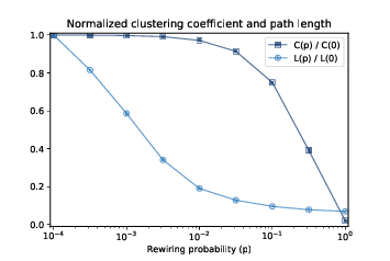
Figure 5.3: Clustering coefficient (C) and characteristic path length (L) for WS graphs with n=1000, k=10, and a range of p.
Now we are ready to replicate the WS experiment, which shows that for a range of values of \(p\), a WS graph has high clustering like a regular graph and short path lengths like a random graph.
We will start with run_one_graph, which takes n, k, and p; it generates a WS graph with the given parameters and computes the mean path length, mpl, and clustering coefficient, cc:
def run_one_graph(n, k, p):
    ws = make_ws_graph(n, k, p)
    mpl = characteristic_path_length(ws)
    cc = clustering_coefficient(ws)
    return mpl, cc
Watts and Strogatz ran their experiment with n=1000 and k=10. With these parameters, run_one_graph takes a few seconds on a typical computer; most of that time is spent computing the mean path length.
Now we need to compute these values for a range of p, using the NumPy function logspace again to compute ps:
ps = np.logspace(-4, 0, 9)
Here’s the function that runs the experiment:
def run_experiment(ps, n=1000, k=10, iters=20):
    res = []
    for p in ps:
            t = [run_one_graph(n, k, p) for _ in range(iters)]
            means = np.array(t).mean(axis=0)
            res.append(means)
    return np.array(res)
For each value of p, we generate 20 random graphs and average the results. Since the return value from run_one_graph is a pair, t is a list of pairs. When we convert it to an array, we get one row for each iteration and columns for L and C. Calling mean with the option axis=0 computes the mean of each column; the result is an array with one row and two columns.
When the loop exits, means is a list of pairs, which we convert to a NumPy array with one row for each value of p and columns for \(L\) and \(C\).
We can extract the columns like this:
L, C = np.transpose(res)
In order to plot L and C on the same axes, we standardize them by dividing by the first element:
L /= L[0]
C /= C[0]
Figure 5.3 shows the results. As p increases, the mean path length drops quickly, because even a small number of randomly rewired edges provide shortcuts between regions of the graph that are far apart in the lattice. On the other hand, removing local links decreases the clustering coefficient much more slowly.
As a result, there is a wide range of p where a WS graph has the properties of a small world graph, high clustering and low path lengths.
And that’s why Watts and Strogatz propose WS graphs as a model for real-world networks that exhibit the small world phenomenon.
- Shortcuts are created during the rewiring process.
- Correct!
- The path does not actual get shorter, It grows
- Try looking at how a rewiring could connect different regions of the graph.
- The edges shrink
- Look again at what is created during the rewiring process.
- All of the above
- Incorrect! Only one of the above is correct.
Q-1: Given that a node returns np.nan, what can you say about the number of edges that node has?