
12.3. Random Perturbation
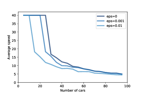
Figure 12.2: Average speed as a function of the number of cars, for three magnitudes of added random noise.
As the number of cars increases, traffic jams become more severe. Figure 12.2 shows the average speed cars are able to achieve, as a function of the number of cars.
The top line shows results with eps=0, that is, with no random variation in speed. With 25 or fewer cars, the spacing between cars is greater than 40, which allows cars to reach and maintain the maximum speed, which is 40. With more than 25 cars, traffic jams form and the average speed drops quickly.
This effect is a direct result of the physics of the simulation, so it should not be surprising. If the length of the road is 1000, the spacing between n cars is 1000/n. And since cars can’t move faster than the space in front of them, the highest average speed we expect is 1000/n or 40, whichever is less.
But that’s the best case scenario. With just a small amount of randomness, things get much worse.
Figure 12.2 also shows results with eps=0.001 and eps=0.01, which correspond to errors in speed of 0.1% and 1%.
With 0.1% errors, the capacity of the highway drops from 25 to 20 (“capacity” means the maximum number of cars that can reach and sustain the speed limit). And with 1% errors, the capacity drops to 10. Ugh.
As one of the exercises at the end of this chapter, you’ll have a chance to design a better driver; that is, you will experiment with different strategies in choose_acceleration and see if you can find driver behaviors that improve average speed.