13.7. Evidence of Evolution

The most inclusive definition of evolution is a change in the distribution of genotypes in a population. Evolution is an aggregate effect: in other words, individuals don’t evolve; populations do.

In this simulation, genotypes are locations in a high-dimensional space, so it is hard to visualize changes in their distribution. However, if the genotypes change, we expect their fitness to change as well. So we will use changes in the distribution of fitness as evidence of evolution. In particular, we’ll look at the mean and standard deviation of fitness over time.

Before we run the simulation, we have to add an Instrument, which is an object that gets updated after each time step, computes a statistic of interest, or “metric”, and stores the result in a sequence we can plot later.

Here is the parent class for all instruments:

class Instrument:
    def __init__(self):
        self.metrics = []

And here’s the definition for MeanFitness, an instrument that computes the mean fitness of the population at each time step:

class MeanFitness(Instrument):
    def update(self, sim):
        mean = np.nanmean(sim.get_fitnesses())
        self.metrics.append(mean)

Now we’re ready to run the simulation. To avoid the effect of random changes in the starting population, we start every simulation with the same set of agents. And to make sure we explore the entire fitness landscape, we start with one agent at every location. Here’s the code that creates the Simulation:

N = 8
fit_land = FitnessLandscape(N)
agents = make_all_agents(fit_land, Agent)
sim = Simulation(fit_land, agents)

make_all_agents creates one Agent for every location; the implementation is in the notebook for this chapter.

Now we can create and add a MeanFitness instrument, run the simulation, and plot the results:

instrument = MeanFitness()
sim.add_instrument(instrument)
sim.run()

Simulation keeps a list of Instrument objects. After each time step it invokes update on each Instrument in the list.

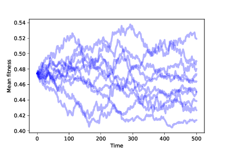
Figure 13.1: Mean fitness over time for 10 simulations with no differential survival or reproduction.

Figure 13.1 shows the result of running this simulation 10 times. The mean fitness of the population drifts up or down at random. Since the distribution of fitness changes over time, we infer that the distribution of phenotypes is also changing. By the most inclusive definition, this random walk is a kind of evolution. But it is not a particularly interesting kind.

In particular, this kind of evolution does not explain how biological species change over time, or how new species appear. The theory of evolution is powerful because it explains phenomena we see in the natural world that seem inexplicable:

• Adaptation: Species interact with their environments in ways that seem too complex, too intricate, and too clever to happen by chance. Many features of natural systems seem as if they were designed.

• Increasing diversity: Over time the number of species on earth has generally increased (despite several periods of mass extinction).

• Increasing complexity: The history of life on earth starts with relatively simple life forms, with more complex organisms appearing later in the geological record.

These are the phenomena we want to explain. So far, our model doesn’t do the job.

Q-1: Evolution is a change in the distribution of genotypes in individuals of a population.

• True
• Incorrect. Please try again.
• False
• Correct. It is a change in the distribution of genotypes in a population. Individuals don’t evolve, populations do.

You have attempted of activities on this page